
 View source on GitHub View source on GitHub |
Overview
이 노트북은 리뷰 텍스트를 사용하여 영화 리뷰를 긍정적 또는 부정적으로 분류합니다. 중요하고도 널리 적용 가능한 머신러닝 문제인 이진 분류의 예입니다.
주어진 입력으로부터 그래프를 빌드하여 이 노트북에서 그래프 정규화를 사용하는 방법을 보여줄 것입니다. 입력에 명시적 그래프가 포함되어 있지 않을 때 Neural Structured Learning(NSL) 프레임워크를 사용하여 그래프 정규화 모델을 빌드하는 일반적인 방법은 다음과 같습니다.
- 입력에서 각 텍스트 샘플에 대한 임베딩을 만듭니다. word2vec, Swivel, BERT 등과 같은 사전 훈련된 모델을 사용하여 수행할 수 있습니다.
- 'L2' 거리, 'cosine' 거리 등과 같은 유사성 메트릭을 사용하여 이러한 임베딩을 기반으로 그래프를 빌드합니다. 그래프에서 노드는 샘플에 해당하고, 그래프에서 간선은 샘플 쌍 간의 유사성에 해당합니다.
- 위의 합성 그래프와 샘플 특성에서 훈련 데이터를 생성합니다. 결과 훈련 데이터에는 원래 노드 특성 외에도 이웃 특성이 포함됩니다.
- Keras 순차, 함수형 또는 서브 클래스 API를 사용하여 신경망을 기본 모델로 만듭니다.
- NSL 프레임워크에서 제공하는 GraphRegularization 래퍼 클래스로 기본 모델을 래핑하여 새 그래프 Keras 모델을 만듭니다. 이 새로운 모델은 훈련 목표에서 그래프 정규화 손실을 정규화 항으로 포함합니다.
- 그래프 Keras 모델을 훈련하고 평가합니다.
참고: 독자가 이 튜토리얼을 진행하는 데 약 1시간이 소요될 것으로 예상됩니다.
요구 사항
- Neural Structured Learning 패키지를 설치합니다.
- tensorflow-hub를 설치합니다.
pip install --quiet neural-structured-learningpip install --quiet tensorflow-hub
종속성 및 가져오기
import matplotlib.pyplot as plt
import numpy as np

import neural_structured_learning as nsl

import tensorflow as tf
import tensorflow_hub as hub

# Resets notebook state
tf.keras.backend.clear_session()

print("Version: ", tf.__version__)
print("Eager mode: ", tf.executing_eagerly())
print("Hub version: ", hub.__version__)
print(
    "GPU is",
    "available" if tf.config.list_physical_devices("GPU") else "NOT AVAILABLE")
Version:  2.6.0
Eager mode:  True
Hub version:  0.12.0
GPU is available
IMDB 데이터세트
IMDB 데이터세트에는 인터넷 영화 데이터베이스에서 가져온 50,000개의 영화 리뷰 텍스트가 포함되어 있습니다. 훈련용 리뷰 25,000개와 테스트용 리뷰 25,000개로 나뉩니다. 훈련 및 테스트 세트는 균형을 이룹니다. 즉, 동일한 수의 긍정적인 리뷰와 부정적인 리뷰가 포함되어 있습니다.
이 튜토리얼에서는 IMDB 데이터세트의 전처리된 버전을 사용합니다.
전처리된 IMDB 데이터세트 다운로드하기
IMDB 데이터세트는 TensorFlow와 함께 패키지로 제공됩니다. 리뷰(단어의 시퀀스)가 정수의 시퀀스로 변환되도록 사전 처리되었으며, 각 정수는 사전에서 특정 단어를 나타냅니다.
다음 코드는 IMDB 데이터세트를 다운로드합니다(또는 이미 다운로드된 경우, 캐시된 사본을 사용합니다).
imdb = tf.keras.datasets.imdb
(pp_train_data, pp_train_labels), (pp_test_data, pp_test_labels) = (
    imdb.load_data(num_words=10000))
Downloading data from https://storage.googleapis.com/tensorflow/tf-keras-datasets/imdb.npz
17465344/17464789 [==============================] - 0s 0us/step
17473536/17464789 [==============================] - 0s 0us/step
인수 num_words=10000은 훈련 데이터에서 가장 자주 발생하는 단어 10,000개를 유지합니다. 어휘의 크기를 관리할 수 있도록 희귀한 단어는 버립니다.
데이터 탐색하기
잠시 시간을 내어 데이터 형식을 살펴보겠습니다. 데이터세트는 사전 처리됩니다. 각 예는 영화 리뷰의 단어를 나타내는 정수 배열입니다. 각 레이블은 0 또는 1의 정수 값입니다. 여기서 0은 부정적인 리뷰이고, 1은 긍정적인 리뷰입니다.
print('Training entries: {}, labels: {}'.format(
    len(pp_train_data), len(pp_train_labels)))
training_samples_count = len(pp_train_data)
Training entries: 25000, labels: 25000
리뷰 텍스트는 정수로 변환되었으며, 각 정수는 사전에서 특정 단어를 나타냅니다. 첫 번째 리뷰는 다음과 같습니다.
print(pp_train_data[0])
[1, 14, 22, 16, 43, 530, 973, 1622, 1385, 65, 458, 4468, 66, 3941, 4, 173, 36, 256, 5, 25, 100, 43, 838, 112, 50, 670, 2, 9, 35, 480, 284, 5, 150, 4, 172, 112, 167, 2, 336, 385, 39, 4, 172, 4536, 1111, 17, 546, 38, 13, 447, 4, 192, 50, 16, 6, 147, 2025, 19, 14, 22, 4, 1920, 4613, 469, 4, 22, 71, 87, 12, 16, 43, 530, 38, 76, 15, 13, 1247, 4, 22, 17, 515, 17, 12, 16, 626, 18, 2, 5, 62, 386, 12, 8, 316, 8, 106, 5, 4, 2223, 5244, 16, 480, 66, 3785, 33, 4, 130, 12, 16, 38, 619, 5, 25, 124, 51, 36, 135, 48, 25, 1415, 33, 6, 22, 12, 215, 28, 77, 52, 5, 14, 407, 16, 82, 2, 8, 4, 107, 117, 5952, 15, 256, 4, 2, 7, 3766, 5, 723, 36, 71, 43, 530, 476, 26, 400, 317, 46, 7, 4, 2, 1029, 13, 104, 88, 4, 381, 15, 297, 98, 32, 2071, 56, 26, 141, 6, 194, 7486, 18, 4, 226, 22, 21, 134, 476, 26, 480, 5, 144, 30, 5535, 18, 51, 36, 28, 224, 92, 25, 104, 4, 226, 65, 16, 38, 1334, 88, 12, 16, 283, 5, 16, 4472, 113, 103, 32, 15, 16, 5345, 19, 178, 32]
영화 리뷰는 길이가 다를 수 있습니다. 아래 코드는 첫 번째 및 두 번째 리뷰의 단어 수를 보여줍니다. 신경망에 대한 입력은 길이가 같아야 하므로 나중에 이 문제를 해결해야 합니다.
len(pp_train_data[0]), len(pp_train_data[1])
(218, 189)
정수를 다시 단어로 변환하기
정수를 해당 텍스트로 다시 변환하는 방법을 아는 것이 유용할 수 있습니다. 여기에서는 정수 대 문자열 매핑을 포함하는 사전 객체를 쿼리하는 도우미 함수를 만듭니다.
def build_reverse_word_index():
  # A dictionary mapping words to an integer index
  word_index = imdb.get_word_index()

  # The first indices are reserved
  word_index = {k: (v + 3) for k, v in word_index.items()}
  word_index['<PAD>'] = 0
  word_index['<START>'] = 1
  word_index['<UNK>'] = 2  # unknown
  word_index['<UNUSED>'] = 3
  return dict((value, key) for (key, value) in word_index.items())

reverse_word_index = build_reverse_word_index()

def decode_review(text):
  return ' '.join([reverse_word_index.get(i, '?') for i in text])
Downloading data from https://storage.googleapis.com/tensorflow/tf-keras-datasets/imdb_word_index.json
1646592/1641221 [==============================] - 0s 0us/step
1654784/1641221 [==============================] - 0s 0us/step
이제 decode_review 함수를 사용하여 첫 번째 리뷰의 텍스트를 표시할 수 있습니다.
decode_review(pp_train_data[0])
"<START> this film was just brilliant casting location scenery story direction everyone's really suited the part they played and you could just imagine being there robert <UNK> is an amazing actor and now the same being director <UNK> father came from the same scottish island as myself so i loved the fact there was a real connection with this film the witty remarks throughout the film were great it was just brilliant so much that i bought the film as soon as it was released for <UNK> and would recommend it to everyone to watch and the fly fishing was amazing really cried at the end it was so sad and you know what they say if you cry at a film it must have been good and this definitely was also <UNK> to the two little boy's that played the <UNK> of norman and paul they were just brilliant children are often left out of the <UNK> list i think because the stars that play them all grown up are such a big profile for the whole film but these children are amazing and should be praised for what they have done don't you think the whole story was so lovely because it was true and was someone's life after all that was shared with us all"
그래프 구성
그래프 구성에는 텍스트 샘플에 대한 임베딩을 만든 다음 유사성 함수를 사용하여 임베딩을 비교하는 것이 포함됩니다.
계속 진행하기 전에 먼저 이 튜토리얼에서 만든 아티팩트를 저장할 디렉터리를 만듭니다.
mkdir -p /tmp/imdb샘플 임베딩 만들기
사전 훈련된 Swivel 임베딩을 사용하여 입력의 각 샘플에 대해 tf.train.Example 형식으로 임베딩을 만듭니다. 각 샘플의 ID를 나타내는 추가 특성과 함께 결과 임베딩을 TFRecord 형식으로 저장합니다. 나중에 그래프의 해당 노드와 샘플 임베딩을 일치시킬 수 있는 중요한 작업입니다.
pretrained_embedding = 'https://tfhub.dev/google/tf2-preview/gnews-swivel-20dim/1'

hub_layer = hub.KerasLayer(
    pretrained_embedding, input_shape=[], dtype=tf.string, trainable=True)
def _int64_feature(value):
  """Returns int64 tf.train.Feature."""
  return tf.train.Feature(int64_list=tf.train.Int64List(value=value.tolist()))


def _bytes_feature(value):
  """Returns bytes tf.train.Feature."""
  return tf.train.Feature(
      bytes_list=tf.train.BytesList(value=[value.encode('utf-8')]))


def _float_feature(value):
  """Returns float tf.train.Feature."""
  return tf.train.Feature(float_list=tf.train.FloatList(value=value.tolist()))


def create_embedding_example(word_vector, record_id):
  """Create tf.Example containing the sample's embedding and its ID."""

  text = decode_review(word_vector)

  # Shape = [batch_size,].
  sentence_embedding = hub_layer(tf.reshape(text, shape=[-1,]))

  # Flatten the sentence embedding back to 1-D.
  sentence_embedding = tf.reshape(sentence_embedding, shape=[-1])

  features = {
      'id': _bytes_feature(str(record_id)),
      'embedding': _float_feature(sentence_embedding.numpy())
  }
  return tf.train.Example(features=tf.train.Features(feature=features))


def create_embeddings(word_vectors, output_path, starting_record_id):
  record_id = int(starting_record_id)
  with tf.io.TFRecordWriter(output_path) as writer:
    for word_vector in word_vectors:
      example = create_embedding_example(word_vector, record_id)
      record_id = record_id + 1
      writer.write(example.SerializeToString())
  return record_id


# Persist TF.Example features containing embeddings for training data in
# TFRecord format.
create_embeddings(pp_train_data, '/tmp/imdb/embeddings.tfr', 0)
25000
그래프 빌드하기
이제 샘플 임베딩이 있으므로 이를 사용하여 유사성 그래프를 빌드합니다. 즉, 이 그래프에서 노드는 샘플에 해당하고, 이 그래프에서 간선은 노드 쌍 간의 유사성에 해당합니다.
Neural Structured Learning은 샘플 임베딩을 기반으로 그래프를 빌드하는 그래프 작성 라이브러리를 제공합니다. 코사인 유사성을 유사성 척도로 사용하여 임베딩을 비교하고 그 사이에 간선을 만듭니다. 또한, 최종 그래프에서 유사하지 않은 간선을 삭제하는 데 사용할 수 있는 유사성 임계값을 지정할 수 있습니다. 이 예에서는 유사성 임계값으로 0.99를 사용하고 임의의 시드로 12345를 사용하면 429,415개의 양방향 간선이 있는 그래프가 생성됩니다. 여기서는 그래프 작성의 속도를 높이기 위해 그래프 빌더의 locality-sensitive hashing(LSH) 지원을 사용하고 있습니다. 그래프 빌더의 LSH 지원을 사용하는 방법에 대한 자세한 내용은 build_graph_from_config API 설명서를 참조하세요.
graph_builder_config = nsl.configs.GraphBuilderConfig(
    similarity_threshold=0.99, lsh_splits=32, lsh_rounds=15, random_seed=12345)
nsl.tools.build_graph_from_config(['/tmp/imdb/embeddings.tfr'],
                                  '/tmp/imdb/graph_99.tsv',
                                  graph_builder_config)
각 양방향 간선은 출력 TSV 파일에서 두 개의 방향 있는 간선으로 표시되므로 파일에는 총 429,415 * 2 = 858,830개 라인이 포함됩니다.
wc -l /tmp/imdb/graph_99.tsv858828 /tmp/imdb/graph_99.tsv
참고: 그래프 품질과 더 나아가 임베딩 품질은 그래프 정규화에 매우 중요합니다. 이 노트북에서는 Swivel 임베딩을 사용했지만, 예를 들어 BERT 임베딩을 사용하면 리뷰 의미 체계를 더 정확하게 파악할 수 있습니다. 사용자가 원하는 임베딩을 필요에 따라 사용할 것을 권장합니다.
샘플 특성
tf.train.Example 형식을 사용하여 문제의 샘플 특성을 만들고 TFRecord 형식으로 유지합니다. 각 샘플에는 다음 3가지 특성이 포함됩니다.
- id: 샘플의 노드 ID입니다.
- words: 단어 ID를 포함하는 int64 목록입니다.
- label: 리뷰의 대상 클래스를 식별하는 싱글톤 int64입니다.
def create_example(word_vector, label, record_id):
  """Create tf.Example containing the sample's word vector, label, and ID."""
  features = {
      'id': _bytes_feature(str(record_id)),
      'words': _int64_feature(np.asarray(word_vector)),
      'label': _int64_feature(np.asarray([label])),
  }
  return tf.train.Example(features=tf.train.Features(feature=features))

def create_records(word_vectors, labels, record_path, starting_record_id):
  record_id = int(starting_record_id)
  with tf.io.TFRecordWriter(record_path) as writer:
    for word_vector, label in zip(word_vectors, labels):
      example = create_example(word_vector, label, record_id)
      record_id = record_id + 1
      writer.write(example.SerializeToString())
  return record_id

# Persist TF.Example features (word vectors and labels) for training and test
# data in TFRecord format.
next_record_id = create_records(pp_train_data, pp_train_labels,
                                '/tmp/imdb/train_data.tfr', 0)
create_records(pp_test_data, pp_test_labels, '/tmp/imdb/test_data.tfr',
               next_record_id)
50000
그래프 이웃으로 훈련 데이터 보강하기
샘플 특성과 합성된 그래프가 있으므로 Neural Structured Learning을 위한 증강 훈련 데이터를 생성할 수 있습니다. NSL 프레임워크는 그래프 정규화를 위한 최종 훈련 데이터를 생성하기 위해 그래프와 샘플 특성을 결합하는 라이브러리를 제공합니다. 결과 훈련 데이터에는 원본 샘플 특성과 해당 이웃의 특성이 포함됩니다.
이 튜토리얼에서는 방향 없는 간선을 고려하고 샘플당 최대 3개의 이웃을 사용하여 그래프 이웃으로 훈련 데이터를 보강합니다.
nsl.tools.pack_nbrs(
    '/tmp/imdb/train_data.tfr',
    '',
    '/tmp/imdb/graph_99.tsv',
    '/tmp/imdb/nsl_train_data.tfr',
    add_undirected_edges=True,
    max_nbrs=3)
기본 모델
이제 그래프 정규화 없이 기본 모델을 빌드할 준비가 되었습니다. 이 모델을 빌드하기 위해 그래프를 빌드하는 데 사용된 임베딩을 사용하거나 분류 작업과 함께 새로운 임베딩을 공동으로 학습할 수 있습니다. 이 노트북의 목적을 위해 후자를 수행합니다.
전역 변수
NBR_FEATURE_PREFIX = 'NL_nbr_'
NBR_WEIGHT_SUFFIX = '_weight'
하이퍼 매개변수
HParams의 인스턴스를 사용하여 훈련 및 평가에 사용되는 다양한 하이퍼 매개변수 및 상수를 포함합니다. 아래에서 각각에 대해 간략하게 설명합니다.
num_classes: 긍정과 부정의 두 가지 클래스가 있습니다.
max_seq_length: 이 예제에서 각 영화 리뷰에서 고려되는 최대 단어 수입니다.
vocab_size: 이 예제에서 고려한 어휘의 크기입니다.
distance_type: 샘플을 이웃으로 정규화하는 데 사용되는 거리 메트릭입니다.
graph_regularization_multiplier: 전체 손실 함수에서 그래프 정규화 항의 상대적 가중치를 제어합니다.
num_neighbors: 그래프 정규화에 사용되는 이웃의 수입니다. 이 값은
nsl.tools.pack_nbrs를 호출할 때 위에서 사용된max_nbrs인수와 같거나 작아야 합니다.num_fc_units: 신경망의 완전 연결 레이어에 있는 단위의 수입니다.
train_epochs: 훈련 epoch의 수입니다.
batch_size: 훈련 및 평가에 사용되는 배치 크기입니다.
eval_steps: 평가가 완료된 것으로 간주하기 전에 처리할 배치의 수입니다.
None으로 설정하면, 테스트 세트의 모든 인스턴스가 평가됩니다.
class HParams(object):
  """Hyperparameters used for training."""
  def __init__(self):
    ### dataset parameters
    self.num_classes = 2
    self.max_seq_length = 256
    self.vocab_size = 10000
    ### neural graph learning parameters
    self.distance_type = nsl.configs.DistanceType.L2
    self.graph_regularization_multiplier = 0.1
    self.num_neighbors = 2
    ### model architecture
    self.num_embedding_dims = 16
    self.num_lstm_dims = 64
    self.num_fc_units = 64
    ### training parameters
    self.train_epochs = 10
    self.batch_size = 128
    ### eval parameters
    self.eval_steps = None  # All instances in the test set are evaluated.

HPARAMS = HParams()
데이터 준비하기
리뷰(정수의 배열)는 신경망에 공급되기 전에 텐서로 변환되어야 합니다. 이 변환은 다음 두 가지 방법으로 수행할 수 있습니다.
배열을 원-핫 인코딩과 유사하게 단어 발생을 나타내는
0및1의 벡터로 변환합니다. 예를 들어, 시퀀스[3, 5]는 1인 인덱스3및5를 제외하고 모두 0인10000차원 벡터가 됩니다. 그런 다음 이를 부동 소수점 벡터 데이터를 처리할 수 있는 네트워크의 첫 번째 레이어인Dense레이어로 만듭니다. 하지만 이 접근 방식은 메모리 집약적이므로num_words * num_reviews크기의 행렬이 필요합니다.또는 배열을 패딩하여 모두 같은 길이를 갖도록 한 다음 형상
max_length * num_reviews의 정수 텐서를 생성할 수 있습니다. 이 형상을 처리할 수 있는 임베딩 레이어를 네트워크의 첫 번째 레이어로 사용할 수 있습니다.
이 튜토리얼에서는 두 번째 접근 방식을 사용합니다.
영화 리뷰는 길이가 같아야 하므로 아래 정의된 pad_sequence 함수를 사용하여 길이를 표준화합니다.
def make_dataset(file_path, training=False):
  """Creates a `tf.data.TFRecordDataset`.

  Args:
    file_path: Name of the file in the `.tfrecord` format containing
      `tf.train.Example` objects.
    training: Boolean indicating if we are in training mode.

  Returns:
    An instance of `tf.data.TFRecordDataset` containing the `tf.train.Example`
    objects.
  """

  def pad_sequence(sequence, max_seq_length):
    """Pads the input sequence (a `tf.SparseTensor`) to `max_seq_length`."""
    pad_size = tf.maximum([0], max_seq_length - tf.shape(sequence)[0])
    padded = tf.concat(
        [sequence.values,
         tf.fill((pad_size), tf.cast(0, sequence.dtype))],
        axis=0)
    # The input sequence may be larger than max_seq_length. Truncate down if
    # necessary.
    return tf.slice(padded, [0], [max_seq_length])

  def parse_example(example_proto):
    """Extracts relevant fields from the `example_proto`.

    Args:
      example_proto: An instance of `tf.train.Example`.

    Returns:
      A pair whose first value is a dictionary containing relevant features
      and whose second value contains the ground truth labels.
    """
    # The 'words' feature is a variable length word ID vector.
    feature_spec = {
        'words': tf.io.VarLenFeature(tf.int64),
        'label': tf.io.FixedLenFeature((), tf.int64, default_value=-1),
    }
    # We also extract corresponding neighbor features in a similar manner to
    # the features above during training.
    if training:
      for i in range(HPARAMS.num_neighbors):
        nbr_feature_key = '{}{}_{}'.format(NBR_FEATURE_PREFIX, i, 'words')
        nbr_weight_key = '{}{}{}'.format(NBR_FEATURE_PREFIX, i,
                                         NBR_WEIGHT_SUFFIX)
        feature_spec[nbr_feature_key] = tf.io.VarLenFeature(tf.int64)

        # We assign a default value of 0.0 for the neighbor weight so that
        # graph regularization is done on samples based on their exact number
        # of neighbors. In other words, non-existent neighbors are discounted.
        feature_spec[nbr_weight_key] = tf.io.FixedLenFeature(
            [1], tf.float32, default_value=tf.constant([0.0]))

    features = tf.io.parse_single_example(example_proto, feature_spec)

    # Since the 'words' feature is a variable length word vector, we pad it to a
    # constant maximum length based on HPARAMS.max_seq_length
    features['words'] = pad_sequence(features['words'], HPARAMS.max_seq_length)
    if training:
      for i in range(HPARAMS.num_neighbors):
        nbr_feature_key = '{}{}_{}'.format(NBR_FEATURE_PREFIX, i, 'words')
        features[nbr_feature_key] = pad_sequence(features[nbr_feature_key],
                                                 HPARAMS.max_seq_length)

    labels = features.pop('label')
    return features, labels

  dataset = tf.data.TFRecordDataset([file_path])
  if training:
    dataset = dataset.shuffle(10000)
  dataset = dataset.map(parse_example)
  dataset = dataset.batch(HPARAMS.batch_size)
  return dataset


train_dataset = make_dataset('/tmp/imdb/nsl_train_data.tfr', True)
test_dataset = make_dataset('/tmp/imdb/test_data.tfr')
모델 빌드하기
신경망은 레이어를 쌓아서 생성됩니다. 이를 위해서는 두 가지 주요 아키텍처 결정이 필요합니다.
- 모델에서 사용할 레이어는 몇 개입니까?
- 각 레이어에 사용할 숨겨진 단위는 몇 개입니까?
이 예제에서 입력 데이터는 단어 인덱스의 배열로 구성됩니다. 예측할 레이블은 0 또는 1입니다.
이 튜토리얼에서는 양방향 LSTM을 기본 모델로 사용합니다.
# This function exists as an alternative to the bi-LSTM model used in this
# notebook.
def make_feed_forward_model():
  """Builds a simple 2 layer feed forward neural network."""
  inputs = tf.keras.Input(
      shape=(HPARAMS.max_seq_length,), dtype='int64', name='words')
  embedding_layer = tf.keras.layers.Embedding(HPARAMS.vocab_size, 16)(inputs)
  pooling_layer = tf.keras.layers.GlobalAveragePooling1D()(embedding_layer)
  dense_layer = tf.keras.layers.Dense(16, activation='relu')(pooling_layer)
  outputs = tf.keras.layers.Dense(1, activation='sigmoid')(dense_layer)
  return tf.keras.Model(inputs=inputs, outputs=outputs)


def make_bilstm_model():
  """Builds a bi-directional LSTM model."""
  inputs = tf.keras.Input(
      shape=(HPARAMS.max_seq_length,), dtype='int64', name='words')
  embedding_layer = tf.keras.layers.Embedding(HPARAMS.vocab_size,
                                              HPARAMS.num_embedding_dims)(
                                                  inputs)
  lstm_layer = tf.keras.layers.Bidirectional(
      tf.keras.layers.LSTM(HPARAMS.num_lstm_dims))(
          embedding_layer)
  dense_layer = tf.keras.layers.Dense(
      HPARAMS.num_fc_units, activation='relu')(
          lstm_layer)
  outputs = tf.keras.layers.Dense(1, activation='sigmoid')(dense_layer)
  return tf.keras.Model(inputs=inputs, outputs=outputs)


# Feel free to use an architecture of your choice.
model = make_bilstm_model()
model.summary()
Model: "model"
_________________________________________________________________
Layer (type)                 Output Shape              Param #
=================================================================
words (InputLayer)           [(None, 256)]             0
_________________________________________________________________
embedding (Embedding)        (None, 256, 16)           160000
_________________________________________________________________
bidirectional (Bidirectional (None, 128)               41472
_________________________________________________________________
dense (Dense)                (None, 64)                8256
_________________________________________________________________
dense_1 (Dense)              (None, 1)                 65
=================================================================
Total params: 209,793
Trainable params: 209,793
Non-trainable params: 0
_________________________________________________________________
레이어는 효과적으로 쌓여 순차적으로 분류자를 빌드합니다.
- 첫 번째 레이어는 정수로 인코딩된 어휘를 사용하는
Input레이어입니다. - 다음 레이어는 정수로 인코딩된 어휘를 사용하여 각 단어 인덱스에 대한 임베딩 벡터를 조회하는
Embedding레이어입니다. 이러한 벡터는 모델 훈련을 통해 학습됩니다. 벡터는 출력 배열에 차원을 추가합니다. 결과 차원은(batch, sequence, embedding)입니다. - 다음으로 양방향 LSTM 레이어는 각 예제에 대해 고정 길이 출력 벡터를 반환합니다.
- 이 고정 길이 출력 벡터는 64개의 숨겨진 단위가 있는 완전 연결(
Dense) 레이어를 통해 파이프됩니다. - 마지막 레이어는 단일 출력 노드와 조밀하게 연결됩니다.
sigmoid활성화 함수를 사용하면, 이 값은 확률 또는 신뢰 수준을 나타내는 0과 1 사이의 부동 소수점입니다.
숨겨진 단위
위의 모델에는 입력과 출력 사이에 두 개의 중간 또는 "숨겨진" 레이어가 있으며, Embedding 레이어는 제외됩니다. 출력(단위, 노드 또는 뉴런)의 수는 레이어에 대한 표현 공간의 차원입니다. 즉, 내부 표현을 학습할 때 네트워크에서 허용되는 자유의 정도입니다.
모델에 더 많은 숨겨진 단위(고차원 표현 공간) 및/또는 더 많은 레이어가 있는 경우, 네트워크는 더 복잡한 표현을 학습할 수 있습니다. 그러나 이는 네트워크를 계산적으로 더 비싸게 만들고, 원치 않는 패턴(훈련 데이터에서는 성능을 향상하지만 테스트 데이터에서는 그렇지 않은 패턴)을 학습하게 됩니다. 이를 과대적합이라고 합니다.
손실 함수 및 옵티마이저
모델에는 훈련을 위한 손실 함수와 옵티마이저가 필요합니다. 이진 분류 문제이고 모델이 확률(시그모이드 활성화가 있는 단일 단위 레이어)을 출력하므로 binary_crossentropy 손실 함수를 사용합니다.
model.compile(
    optimizer='adam', loss='binary_crossentropy', metrics=['accuracy'])
검증 세트 만들기
훈련할 때, 이전에 본 적이 없는 데이터에 대한 모델의 정확성을 확인하려고 합니다. 원래 훈련 데이터의 일부를 구분하여 검증 세트를 만듭니다. (왜 지금 테스트 세트를 사용하지 않을까요? 목표는 훈련 데이터만 사용하여 모델을 개발하고 조정한 다음, 테스트 데이터를 한 번만 사용하여 정확성을 평가하는 것입니다.)
이 튜토리얼에서는 초기 훈련 샘플의 약 10%(25000의 10%)를 훈련용 데이터로 레이블 지정하고 나머지는 검증 데이터로 사용합니다. 초기 훈련/테스트 분할이 50/50(각각 25000개 샘플)이므로 현재 유효한 훈련/검증/테스트 분할은 5/45/50입니다.
'train_dataset'는 이미 일괄 처리되고 셔플되었습니다.
validation_fraction = 0.9
validation_size = int(validation_fraction *
                      int(training_samples_count / HPARAMS.batch_size))
print(validation_size)
validation_dataset = train_dataset.take(validation_size)
train_dataset = train_dataset.skip(validation_size)
175
모델을 훈련 시키십시오
미니 배치로 모델을 훈련합니다. 훈련하는 동안 검증 세트에 대해 모델의 손실과 정확성을 모니터링합니다.
history = model.fit(
    train_dataset,
    validation_data=validation_dataset,
    epochs=HPARAMS.train_epochs,
    verbose=1)
Epoch 1/10
/tmpfs/src/tf_docs_env/lib/python3.7/site-packages/keras/engine/functional.py:585: UserWarning: Input dict contained keys ['NL_nbr_0_words', 'NL_nbr_1_words', 'NL_nbr_0_weight', 'NL_nbr_1_weight'] which did not match any model input. They will be ignored by the model.
  [n for n in tensors.keys() if n not in ref_input_names])
21/21 [==============================] - 8s 140ms/step - loss: 0.6930 - accuracy: 0.5069 - val_loss: 0.6928 - val_accuracy: 0.5019
Epoch 2/10
21/21 [==============================] - 3s 111ms/step - loss: 0.6923 - accuracy: 0.5119 - val_loss: 0.6917 - val_accuracy: 0.5317
Epoch 3/10
21/21 [==============================] - 3s 111ms/step - loss: 0.6827 - accuracy: 0.5892 - val_loss: 0.6899 - val_accuracy: 0.5424
Epoch 4/10
21/21 [==============================] - 3s 111ms/step - loss: 0.6589 - accuracy: 0.6550 - val_loss: 0.6445 - val_accuracy: 0.6614
Epoch 5/10
21/21 [==============================] - 3s 112ms/step - loss: 0.6446 - accuracy: 0.6654 - val_loss: 0.6356 - val_accuracy: 0.6889
Epoch 6/10
21/21 [==============================] - 3s 110ms/step - loss: 0.6146 - accuracy: 0.7035 - val_loss: 0.5842 - val_accuracy: 0.7102
Epoch 7/10
21/21 [==============================] - 3s 111ms/step - loss: 0.4995 - accuracy: 0.7665 - val_loss: 0.4513 - val_accuracy: 0.7982
Epoch 8/10
21/21 [==============================] - 3s 110ms/step - loss: 0.4300 - accuracy: 0.8150 - val_loss: 0.4427 - val_accuracy: 0.7969
Epoch 9/10
21/21 [==============================] - 3s 113ms/step - loss: 0.3854 - accuracy: 0.8342 - val_loss: 0.3523 - val_accuracy: 0.8530
Epoch 10/10
21/21 [==============================] - 3s 112ms/step - loss: 0.3240 - accuracy: 0.8754 - val_loss: 0.3240 - val_accuracy: 0.8708
모델 평가하기
이제 모델의 성능을 살펴보겠습니다. 두 개의 값, 즉 손실(오류를 나타내는 숫자, 낮은 값이 더 좋음) 및 정확성이 반환됩니다.
results = model.evaluate(test_dataset, steps=HPARAMS.eval_steps)
print(results)
196/196 [==============================] - 3s 10ms/step - loss: 0.3884 - accuracy: 0.8370
[0.38840407133102417, 0.8370400071144104]
시간 경과에 따른 정확성/손실 그래프 생성하기
model.fit()은 훈련 중에 발생한 모든 것을 가진 사전을 포함하는 History 객체를 반환합니다.
history_dict = history.history
history_dict.keys()
dict_keys(['loss', 'accuracy', 'val_loss', 'val_accuracy'])
4개의 항목이 있습니다. 훈련 및 검증 중에 모니터링되는 각 메트릭에 대해 하나씩 있습니다. 이들 항목을 사용하여 비교를 위한 훈련 및 검증 손실과 훈련 및 검증 정확성을 플롯할 수 있습니다.
acc = history_dict['accuracy']
val_acc = history_dict['val_accuracy']
loss = history_dict['loss']
val_loss = history_dict['val_loss']
epochs = range(1, len(acc) + 1)
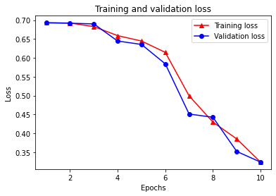
# "-r^" is for solid red line with triangle markers.
plt.plot(epochs, loss, '-r^', label='Training loss')
# "-b0" is for solid blue line with circle markers.
plt.plot(epochs, val_loss, '-bo', label='Validation loss')
plt.title('Training and validation loss')
plt.xlabel('Epochs')
plt.ylabel('Loss')
plt.legend(loc='best')
plt.show()
plt.clf()   # clear figure

plt.plot(epochs, acc, '-r^', label='Training acc')
plt.plot(epochs, val_acc, '-bo', label='Validation acc')
plt.title('Training and validation accuracy')
plt.xlabel('Epochs')
plt.ylabel('Accuracy')
plt.legend(loc='best')

plt.show()
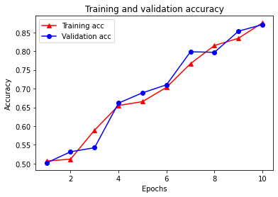
훈련 손실은 각 epoch마다 감소하고 훈련 정확성은 각 epoch마다 증가합니다. 경사 하강 최적화를 사용할 때 이와 같이 예상됩니다. 모든 반복에서 원하는 수량을 최소화해야 합니다.
그래프 정규화
이제 위에서 구축한 기본 모델을 사용하여 그래프 정규화를 시도할 준비가 되었습니다. Neural Structured Learning 프레임워크에서 제공하는 GraphRegularization 래퍼 클래스를 사용하여 그래프 정규화를 포함하도록 기본 (bi-LSTM) 모델을 래핑합니다. 그래프 정규화 모델을 훈련하고 평가하기 위한 나머지 단계는 기본 모델의 단계와 유사합니다.
그래프 정규화 모델 생성하기
그래프 정규화의 점진적 이점을 평가하기 위해 새 기본 모델 인스턴스를 생성합니다. model은 몇 번의 반복으로 이미 훈련되었고, 그래프-정규화 모델을 만들기 위해 이 훈련 모델을 재사용하면 model을 위한 공정한 비교가 되지 않습니다.
# Build a new base LSTM model.
base_reg_model = make_bilstm_model()
# Wrap the base model with graph regularization.
graph_reg_config = nsl.configs.make_graph_reg_config(
    max_neighbors=HPARAMS.num_neighbors,
    multiplier=HPARAMS.graph_regularization_multiplier,
    distance_type=HPARAMS.distance_type,
    sum_over_axis=-1)
graph_reg_model = nsl.keras.GraphRegularization(base_reg_model,
                                                graph_reg_config)
graph_reg_model.compile(
    optimizer='adam', loss='binary_crossentropy', metrics=['accuracy'])
모델 훈련하기
graph_reg_history = graph_reg_model.fit(
    train_dataset,
    validation_data=validation_dataset,
    epochs=HPARAMS.train_epochs,
    verbose=1)
Epoch 1/10
/tmpfs/src/tf_docs_env/lib/python3.7/site-packages/tensorflow/python/framework/indexed_slices.py:449: UserWarning: Converting sparse IndexedSlices(IndexedSlices(indices=Tensor("gradient_tape/GraphRegularization/graph_loss/Reshape_1:0", shape=(None,), dtype=int32), values=Tensor("gradient_tape/GraphRegularization/graph_loss/Reshape:0", shape=(None, 1), dtype=float32), dense_shape=Tensor("gradient_tape/GraphRegularization/graph_loss/Cast:0", shape=(2,), dtype=int32))) to a dense Tensor of unknown shape. This may consume a large amount of memory.
  "shape. This may consume a large amount of memory." % value)
21/21 [==============================] - 10s 189ms/step - loss: 0.6931 - accuracy: 0.4988 - scaled_graph_loss: 1.1141e-06 - val_loss: 0.6926 - val_accuracy: 0.5004
Epoch 2/10
21/21 [==============================] - 3s 139ms/step - loss: 0.6899 - accuracy: 0.5327 - scaled_graph_loss: 2.0430e-05 - val_loss: 0.6844 - val_accuracy: 0.5194
Epoch 3/10
21/21 [==============================] - 3s 143ms/step - loss: 0.6527 - accuracy: 0.6362 - scaled_graph_loss: 9.6421e-04 - val_loss: 0.5461 - val_accuracy: 0.7525
Epoch 4/10
21/21 [==============================] - 3s 142ms/step - loss: 0.5031 - accuracy: 0.7715 - scaled_graph_loss: 0.0074 - val_loss: 0.4108 - val_accuracy: 0.8168
Epoch 5/10
21/21 [==============================] - 3s 143ms/step - loss: 0.3905 - accuracy: 0.8354 - scaled_graph_loss: 0.0158 - val_loss: 0.3452 - val_accuracy: 0.8580
Epoch 6/10
21/21 [==============================] - 3s 144ms/step - loss: 0.3623 - accuracy: 0.8596 - scaled_graph_loss: 0.0186 - val_loss: 0.3074 - val_accuracy: 0.8781
Epoch 7/10
21/21 [==============================] - 3s 144ms/step - loss: 0.3246 - accuracy: 0.8781 - scaled_graph_loss: 0.0201 - val_loss: 0.2957 - val_accuracy: 0.8838
Epoch 8/10
21/21 [==============================] - 3s 143ms/step - loss: 0.2915 - accuracy: 0.8946 - scaled_graph_loss: 0.0211 - val_loss: 0.2680 - val_accuracy: 0.8964
Epoch 9/10
21/21 [==============================] - 3s 146ms/step - loss: 0.2900 - accuracy: 0.8981 - scaled_graph_loss: 0.0236 - val_loss: 0.2595 - val_accuracy: 0.9022
Epoch 10/10
21/21 [==============================] - 3s 143ms/step - loss: 0.2721 - accuracy: 0.9115 - scaled_graph_loss: 0.0233 - val_loss: 0.2524 - val_accuracy: 0.9023
모델 평가하기
graph_reg_results = graph_reg_model.evaluate(test_dataset, steps=HPARAMS.eval_steps)
print(graph_reg_results)
196/196 [==============================] - 3s 10ms/step - loss: 0.3602 - accuracy: 0.8478
[0.36020034551620483, 0.8478400111198425]
Create a graph of accuracy/loss over time
graph_reg_history_dict = graph_reg_history.history
graph_reg_history_dict.keys()
dict_keys(['loss', 'accuracy', 'scaled_graph_loss', 'val_loss', 'val_accuracy'])
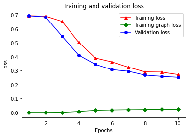
사전에는 훈련 손실, 훈련 정확성, 훈련 그래프 손실, 검증 손실 및 검증 정확성의 총 5개 항목이 있습니다. 비교를 위해 모두 함께 플롯할 수 있습니다. 그래프 손실은 훈련 중에만 계산됩니다.
acc = graph_reg_history_dict['accuracy']
val_acc = graph_reg_history_dict['val_accuracy']
loss = graph_reg_history_dict['loss']
graph_loss = graph_reg_history_dict['scaled_graph_loss']
val_loss = graph_reg_history_dict['val_loss']

epochs = range(1, len(acc) + 1)

plt.clf()   # clear figure

# "-r^" is for solid red line with triangle markers.
plt.plot(epochs, loss, '-r^', label='Training loss')
# "-gD" is for solid green line with diamond markers.
plt.plot(epochs, graph_loss, '-gD', label='Training graph loss')
# "-b0" is for solid blue line with circle markers.
plt.plot(epochs, val_loss, '-bo', label='Validation loss')
plt.title('Training and validation loss')
plt.xlabel('Epochs')
plt.ylabel('Loss')
plt.legend(loc='best')

plt.show()
plt.clf() # clear figure
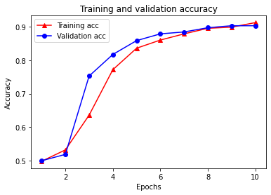
plt.plot(epochs, acc, '-r^', label='Training acc')
plt.plot(epochs, val_acc, '-bo', label='Validation acc')
plt.title('Training and validation accuracy')
plt.xlabel('Epochs')
plt.ylabel('Accuracy')
plt.legend(loc='best')
plt.show()
준감독 학습의 힘
준감독 학습, 보다 구체적으로 이 튜토리얼의 맥락에서 그래프 정규화는 훈련 데이터의 양이 적을 때 정말 강력할 수 있습니다. 훈련 데이터의 부족은 훈련 샘플 간의 유사성을 활용하여 보완되며, 기존 감독 학습에서는 불가능했습니다.
감독 비율을 훈련, 검증, 테스트 샘플을 포함하는 총 샘플 수에 대한 훈련 샘플의 비율로 정의합니다. 이 노트북에서는 기본 모델과 그래프 정규화 모델 모두를 훈련하기 위해 0.05의 감독 비율(즉, 레이블이 지정된 데이터의 5%)을 사용했습니다. 아래 셀에서 감독 비율이 모델 정확성에 미치는 영향을 설명합니다.
# Accuracy values for both the Bi-LSTM model and the feed forward NN model have
# been precomputed for the following supervision ratios.

supervision_ratios = [0.3, 0.15, 0.05, 0.03, 0.02, 0.01, 0.005]

model_tags = ['Bi-LSTM model', 'Feed Forward NN model']
base_model_accs = [[84, 84, 83, 80, 65, 52, 50], [87, 86, 76, 74, 67, 52, 51]]
graph_reg_model_accs = [[84, 84, 83, 83, 65, 63, 50],
                        [87, 86, 80, 75, 67, 52, 50]]

plt.clf()  # clear figure

fig, axes = plt.subplots(1, 2)
fig.set_size_inches((12, 5))

for ax, model_tag, base_model_acc, graph_reg_model_acc in zip(
    axes, model_tags, base_model_accs, graph_reg_model_accs):

  # "-r^" is for solid red line with triangle markers.
  ax.plot(base_model_acc, '-r^', label='Base model')
  # "-gD" is for solid green line with diamond markers.
  ax.plot(graph_reg_model_acc, '-gD', label='Graph-regularized model')
  ax.set_title(model_tag)
  ax.set_xlabel('Supervision ratio')
  ax.set_ylabel('Accuracy(%)')
  ax.set_ylim((25, 100))
  ax.set_xticks(range(len(supervision_ratios)))
  ax.set_xticklabels(supervision_ratios)
  ax.legend(loc='best')

plt.show()
<Figure size 432x288 with 0 Axes>
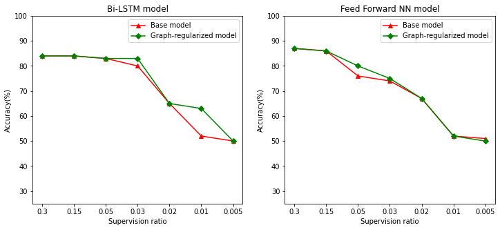
감독 비율이 감소하면 모델 정확성도 감소함을 알 수 있습니다. 이는 사용 된 모델 아키텍처와 관계없이 기본 모델과 그래프 정규화 모델 모두에 해당됩니다. 그러나 그래프 정규화 모델은 두 아키텍처 모두에서 기본 모델보다 더 나은 성능을 발휘합니다. 특히 Bi-LSTM 모델의 경우, 감독 비율이 0.01일 때 그래프 정규화 모델의 정확성은 기본 모델보다 ~20% 높습니다. 이는 주로 훈련 샘플 자체 외에 훈련 샘플 간의 구조적 유사성이 사용되는 그래프 정규화 모델에 대한 준감독 학습 때문입니다.
결론
입력에 명시적 그래프가 포함되지 않은 경우에도 Neural Structured Learning(NSL) 프레임워크를 사용하여 그래프 정규화를 사용하는 방법을 시연했습니다. 리뷰 임베딩을 기반으로 유사성 그래프를 합성한 IMDB 영화 리뷰의 감상 분류 작업을 고려했습니다. 사용자가 다양한 하이퍼 매개변수, 감독의 양 및 다양한 모델 아키텍처를 사용하여 추가로 실험할 것을 권장합니다.