
| |  GitHubでソースを表示 GitHubでソースを表示 | |
概要
レビューのテキストを使用して、正または負としてこのノート分類の映画のレビュー。これは、バイナリ分類、機械学習、問題の重要かつ広く適用の種類の一例です。
与えられた入力からグラフを作成することにより、このノートブックでのグラフ正則化の使用法を示します。入力に明示的なグラフが含まれていない場合に、Neural Structured Learning(NSL)フレームワークを使用してグラフ正則化モデルを構築するための一般的なレシピは、次のとおりです。
- 入力のテキストサンプルごとに埋め込みを作成します。これは、次のような事前に訓練されたモデルで使用して行うことができますword2vec 、スイベル、 BERTなど
- 「L2」距離、「コサイン」距離などの類似性メトリックを使用して、これらの埋め込みに基づいてグラフを作成します。グラフのノードはサンプルに対応し、グラフのエッジはサンプルのペア間の類似性に対応します。
- 上記の合成グラフとサンプル特徴からトレーニングデータを生成します。結果のトレーニングデータには、元のノード機能に加えて隣接機能が含まれます。
- Kerasシーケンシャル、機能、またはサブクラスAPIを使用して、ベースモデルとしてニューラルネットワークを作成します。
- NSLフレームワークによって提供されるGraphRegularizationラッパークラスでベースモデルをラップして、新しいグラフKerasモデルを作成します。この新しいモデルには、トレーニング目標の正則化項としてグラフ正則化損失が含まれます。
- グラフKerasモデルをトレーニングして評価します。
要件
- Neural StructuredLearningパッケージをインストールします。
- tensorflow-hubをインストールします。
pip install --quiet neural-structured-learningpip install --quiet tensorflow-hub
依存関係とインポート
import matplotlib.pyplot as plt
import numpy as np

import neural_structured_learning as nsl

import tensorflow as tf
import tensorflow_hub as hub

# Resets notebook state
tf.keras.backend.clear_session()

print("Version: ", tf.__version__)
print("Eager mode: ", tf.executing_eagerly())
print("Hub version: ", hub.__version__)
print(
    "GPU is",
    "available" if tf.config.list_physical_devices("GPU") else "NOT AVAILABLE")
Version:  2.8.0-rc0
Eager mode:  True
Hub version:  0.12.0
GPU is NOT AVAILABLE
2022-01-05 12:28:32.113752: E tensorflow/stream_executor/cuda/cuda_driver.cc:271] failed call to cuInit: CUDA_ERROR_NO_DEVICE: no CUDA-capable device is detected
IMDBデータセット
IMDBのデータセットは、 50,000から映画のレビューのテキストが含まれ、インターネットムービーデータベースを。これらは、トレーニング用の25,000件のレビューとテスト用の25,000件のレビューに分けられます。トレーニングとテストセットは、それらが正と負のレビューの同じ番号が含ま意味、バランスされています。
このチュートリアルでは、前処理されたバージョンのIMDBデータセットを使用します。
前処理されたIMDBデータセットをダウンロードする
IMDBデータセットはTensorFlowにパッケージ化されています。レビュー(単語のシーケンス)が整数のシーケンスに変換されるように、すでに前処理されています。各整数は、辞書内の特定の単語を表します。
次のコードは、IMDBデータセットをダウンロードします(または、すでにダウンロードされている場合は、キャッシュされたコピーを使用します)。
imdb = tf.keras.datasets.imdb
(pp_train_data, pp_train_labels), (pp_test_data, pp_test_labels) = (
    imdb.load_data(num_words=10000))
Downloading data from https://storage.googleapis.com/tensorflow/tf-keras-datasets/imdb.npz
17465344/17464789 [==============================] - 0s 0us/step
17473536/17464789 [==============================] - 0s 0us/step
引数num_words=10000トレーニングデータのトップ万最も頻繁に出現する単語を保持します。語彙のサイズを管理しやすくするために、まれな単語は破棄されます。
データを調べる
データの形式を理解するために少し時間を取ってみましょう。データセットは前処理されています。各例は、映画レビューの単語を表す整数の配列です。各ラベルは0または1の整数値であり、0は否定的なレビュー、1は肯定的なレビューです。
print('Training entries: {}, labels: {}'.format(
    len(pp_train_data), len(pp_train_labels)))
training_samples_count = len(pp_train_data)
Training entries: 25000, labels: 25000
レビューのテキストは整数に変換されており、各整数は辞書内の特定の単語を表しています。最初のレビューは次のようになります。
print(pp_train_data[0])
[1, 14, 22, 16, 43, 530, 973, 1622, 1385, 65, 458, 4468, 66, 3941, 4, 173, 36, 256, 5, 25, 100, 43, 838, 112, 50, 670, 2, 9, 35, 480, 284, 5, 150, 4, 172, 112, 167, 2, 336, 385, 39, 4, 172, 4536, 1111, 17, 546, 38, 13, 447, 4, 192, 50, 16, 6, 147, 2025, 19, 14, 22, 4, 1920, 4613, 469, 4, 22, 71, 87, 12, 16, 43, 530, 38, 76, 15, 13, 1247, 4, 22, 17, 515, 17, 12, 16, 626, 18, 2, 5, 62, 386, 12, 8, 316, 8, 106, 5, 4, 2223, 5244, 16, 480, 66, 3785, 33, 4, 130, 12, 16, 38, 619, 5, 25, 124, 51, 36, 135, 48, 25, 1415, 33, 6, 22, 12, 215, 28, 77, 52, 5, 14, 407, 16, 82, 2, 8, 4, 107, 117, 5952, 15, 256, 4, 2, 7, 3766, 5, 723, 36, 71, 43, 530, 476, 26, 400, 317, 46, 7, 4, 2, 1029, 13, 104, 88, 4, 381, 15, 297, 98, 32, 2071, 56, 26, 141, 6, 194, 7486, 18, 4, 226, 22, 21, 134, 476, 26, 480, 5, 144, 30, 5535, 18, 51, 36, 28, 224, 92, 25, 104, 4, 226, 65, 16, 38, 1334, 88, 12, 16, 283, 5, 16, 4472, 113, 103, 32, 15, 16, 5345, 19, 178, 32]
映画のレビューは長さが異なる場合があります。以下のコードは、1回目と2回目のレビューの単語数を示しています。ニューラルネットワークへの入力は同じ長さでなければならないため、後でこれを解決する必要があります。
len(pp_train_data[0]), len(pp_train_data[1])
(218, 189)
整数を単語に変換し直します
整数を対応するテキストに戻す方法を知っておくと便利な場合があります。ここでは、整数から文字列へのマッピングを含む辞書オブジェクトをクエリするヘルパー関数を作成します。
def build_reverse_word_index():
  # A dictionary mapping words to an integer index
  word_index = imdb.get_word_index()

  # The first indices are reserved
  word_index = {k: (v + 3) for k, v in word_index.items()}
  word_index['<PAD>'] = 0
  word_index['<START>'] = 1
  word_index['<UNK>'] = 2  # unknown
  word_index['<UNUSED>'] = 3
  return dict((value, key) for (key, value) in word_index.items())

reverse_word_index = build_reverse_word_index()

def decode_review(text):
  return ' '.join([reverse_word_index.get(i, '?') for i in text])
Downloading data from https://storage.googleapis.com/tensorflow/tf-keras-datasets/imdb_word_index.json
1646592/1641221 [==============================] - 0s 0us/step
1654784/1641221 [==============================] - 0s 0us/step
今、私たちは使用することができますdecode_review最初のレビューのためのテキストを表示する機能を:
decode_review(pp_train_data[0])
"<START> this film was just brilliant casting location scenery story direction everyone's really suited the part they played and you could just imagine being there robert <UNK> is an amazing actor and now the same being director <UNK> father came from the same scottish island as myself so i loved the fact there was a real connection with this film the witty remarks throughout the film were great it was just brilliant so much that i bought the film as soon as it was released for <UNK> and would recommend it to everyone to watch and the fly fishing was amazing really cried at the end it was so sad and you know what they say if you cry at a film it must have been good and this definitely was also <UNK> to the two little boy's that played the <UNK> of norman and paul they were just brilliant children are often left out of the <UNK> list i think because the stars that play them all grown up are such a big profile for the whole film but these children are amazing and should be praised for what they have done don't you think the whole story was so lovely because it was true and was someone's life after all that was shared with us all"
グラフの構築
グラフの作成には、テキストサンプルの埋め込みを作成し、類似度関数を使用して埋め込みを比較することが含まれます。
先に進む前に、まず、このチュートリアルで作成されたアーティファクトを格納するディレクトリを作成します。
mkdir -p /tmp/imdb
サンプル埋め込みを作成する
私たちは中に埋め込みを作成するためにpretrainedスイベルの埋め込みを使用しますtf.train.Example入力の各サンプルのためのフォーマット。我々は、中の得られた埋め込み格納するTFRecord各サンプルのIDを表す付加的な特徴と共にフォーマット。これは重要であり、後でサンプルの埋め込みをグラフ内の対応するノードと一致させることができます。
pretrained_embedding = 'https://tfhub.dev/google/tf2-preview/gnews-swivel-20dim/1'

hub_layer = hub.KerasLayer(
    pretrained_embedding, input_shape=[], dtype=tf.string, trainable=True)
def _int64_feature(value):
  """Returns int64 tf.train.Feature."""
  return tf.train.Feature(int64_list=tf.train.Int64List(value=value.tolist()))


def _bytes_feature(value):
  """Returns bytes tf.train.Feature."""
  return tf.train.Feature(
      bytes_list=tf.train.BytesList(value=[value.encode('utf-8')]))


def _float_feature(value):
  """Returns float tf.train.Feature."""
  return tf.train.Feature(float_list=tf.train.FloatList(value=value.tolist()))


def create_embedding_example(word_vector, record_id):
  """Create tf.Example containing the sample's embedding and its ID."""

  text = decode_review(word_vector)

  # Shape = [batch_size,].
  sentence_embedding = hub_layer(tf.reshape(text, shape=[-1,]))

  # Flatten the sentence embedding back to 1-D.
  sentence_embedding = tf.reshape(sentence_embedding, shape=[-1])

  features = {
      'id': _bytes_feature(str(record_id)),
      'embedding': _float_feature(sentence_embedding.numpy())
  }
  return tf.train.Example(features=tf.train.Features(feature=features))


def create_embeddings(word_vectors, output_path, starting_record_id):
  record_id = int(starting_record_id)
  with tf.io.TFRecordWriter(output_path) as writer:
    for word_vector in word_vectors:
      example = create_embedding_example(word_vector, record_id)
      record_id = record_id + 1
      writer.write(example.SerializeToString())
  return record_id


# Persist TF.Example features containing embeddings for training data in
# TFRecord format.
create_embeddings(pp_train_data, '/tmp/imdb/embeddings.tfr', 0)
25000
グラフを作成する
サンプルの埋め込みができたので、それらを使用して類似性グラフを作成します。つまり、このグラフのノードはサンプルに対応し、このグラフのエッジはノードのペア間の類似性に対応します。
Neural Structured Learningは、サンプルの埋め込みに基づいてグラフを作成するためのグラフ作成ライブラリを提供します。これは、使用していますコサイン類似度を、それらの間の埋め込みとビルドエッジを比較するために、類似性尺度として。また、類似性のしきい値を指定することもできます。これを使用して、最終的なグラフから異なるエッジを破棄できます。この例では、類似性のしきい値として0.99を使用し、ランダムシードとして12345を使用すると、429,415の双方向エッジを持つグラフになります。ここでは、ためのグラフビルダーのサポート使用している局所性鋭敏型ハッシュグラフの構築をスピードアップするために(LSH)を。グラフビルダーのLSHのサポートを使用しての詳細については、を参照build_graph_from_config APIドキュメントを。
graph_builder_config = nsl.configs.GraphBuilderConfig(
    similarity_threshold=0.99, lsh_splits=32, lsh_rounds=15, random_seed=12345)
nsl.tools.build_graph_from_config(['/tmp/imdb/embeddings.tfr'],
                                  '/tmp/imdb/graph_99.tsv',
                                  graph_builder_config)
各双方向エッジは、出力TSVファイルの2つの有向エッジで表されるため、ファイルには429,415 * 2 = 858,830の合計行が含まれます。
wc -l /tmp/imdb/graph_99.tsv
858830 /tmp/imdb/graph_99.tsv
サンプル機能
私たちは、使用して我々の問題のためのサンプルの特徴を作成tf.train.Example形式をして、それらを持続TFRecordフォーマット。各サンプルには、次の3つの機能が含まれます。
- ID:サンプルのノードID。
- 単語:単語IDを含むint64型の一覧。
- ラベル:レビューの対象クラスを識別int64型シングルトン。
def create_example(word_vector, label, record_id):
  """Create tf.Example containing the sample's word vector, label, and ID."""
  features = {
      'id': _bytes_feature(str(record_id)),
      'words': _int64_feature(np.asarray(word_vector)),
      'label': _int64_feature(np.asarray([label])),
  }
  return tf.train.Example(features=tf.train.Features(feature=features))

def create_records(word_vectors, labels, record_path, starting_record_id):
  record_id = int(starting_record_id)
  with tf.io.TFRecordWriter(record_path) as writer:
    for word_vector, label in zip(word_vectors, labels):
      example = create_example(word_vector, label, record_id)
      record_id = record_id + 1
      writer.write(example.SerializeToString())
  return record_id

# Persist TF.Example features (word vectors and labels) for training and test
# data in TFRecord format.
next_record_id = create_records(pp_train_data, pp_train_labels,
                                '/tmp/imdb/train_data.tfr', 0)
create_records(pp_test_data, pp_test_labels, '/tmp/imdb/test_data.tfr',
               next_record_id)
50000
グラフネイバーを使用してトレーニングデータを拡張する
サンプルの特徴と合成されたグラフがあるので、ニューラル構造化学習用の拡張トレーニングデータを生成できます。 NSLフレームワークは、グラフとサンプル機能を組み合わせて、グラフの正則化のための最終的なトレーニングデータを生成するためのライブラリを提供します。結果のトレーニングデータには、元のサンプル機能とそれに対応するネイバーの機能が含まれます。
このチュートリアルでは、無向エッジを考慮し、サンプルごとに最大3つのネイバーを使用して、グラフネイバーでトレーニングデータを拡張します。
nsl.tools.pack_nbrs(
    '/tmp/imdb/train_data.tfr',
    '',
    '/tmp/imdb/graph_99.tsv',
    '/tmp/imdb/nsl_train_data.tfr',
    add_undirected_edges=True,
    max_nbrs=3)
ベースモデル
これで、グラフの正則化なしでベースモデルを構築する準備が整いました。このモデルを構築するために、グラフの構築に使用された埋め込みを使用するか、分類タスクと一緒に新しい埋め込みを学習することができます。このノートブックの目的のために、後者を行います。
グローバル変数
NBR_FEATURE_PREFIX = 'NL_nbr_'
NBR_WEIGHT_SUFFIX = '_weight'
ハイパーパラメータ
私たちは、のインスタンスを使用しますHParams訓練し、評価のために使用される様々なハイパーや定数をinclueします。以下に、それぞれについて簡単に説明します。
num_classesは: -正と負の2つのクラスがあります。
max_seq_length:これは、この例では、各映画のレビューから考えられた単語の最大数です。
vocab_size:これは、この例のために考えられた語彙の大きさです。
distance_type:これは隣国でサンプルを正則化するために使用されるメトリックの距離です。
graph_regularization_multiplier:この全体を制御する損失関数のグラフの正則化項の相対重量。
num_neighbors:グラフ正則に使用するネイバーの数。この値が等しいかまたはそれ以下でなければならない
max_nbrs起動時には、上記使用引数nsl.tools.pack_nbrs。num_fc_units:ニューラルネットワークの完全に接続された層のユニット数。
train_epochs:トレーニングエポック数。
BATCH_SIZE:トレーニングや評価に用いるバッチサイズ。
eval_steps:評価をみなし前に処理するバッチの数は完了です。設定した場合
None、テスト・セット内のすべてのインスタンスが評価されます。
class HParams(object):
  """Hyperparameters used for training."""
  def __init__(self):
    ### dataset parameters
    self.num_classes = 2
    self.max_seq_length = 256
    self.vocab_size = 10000
    ### neural graph learning parameters
    self.distance_type = nsl.configs.DistanceType.L2
    self.graph_regularization_multiplier = 0.1
    self.num_neighbors = 2
    ### model architecture
    self.num_embedding_dims = 16
    self.num_lstm_dims = 64
    self.num_fc_units = 64
    ### training parameters
    self.train_epochs = 10
    self.batch_size = 128
    ### eval parameters
    self.eval_steps = None  # All instances in the test set are evaluated.

HPARAMS = HParams()
データを準備する
レビュー(整数の配列)は、ニューラルネットワークに入力される前にテンソルに変換する必要があります。この変換は、いくつかの方法で実行できます。
配列はベクターに変換する
0秒と1ワンホット符号化と同様の指示語の出現、。例えば、配列は[3, 5]となる10000インデックスを除くすべてゼロである次元ベクトル3及び5のものです。次に、この私たちのネットワーク内の第一層せるDense層浮動小数点ベクトルデータを扱うことができます。このアプローチは、必要な、しかし、メモリ集約的でありnum_words * num_reviewsサイズの行列を。それらは全て同じ長さを有しているので代わりに、我々は、パッドアレイは、次いで、形状の整数テンソル作成でき
max_length * num_reviews。この形状を処理できる埋め込みレイヤーをネットワークの最初のレイヤーとして使用できます。
このチュートリアルでは、2番目のアプローチを使用します。
映画のレビューは、同じ長さでなければならないので、我々は、使用するpad_sequence長さを標準化するには、以下の定義関数を。
def make_dataset(file_path, training=False):
  """Creates a `tf.data.TFRecordDataset`.

  Args:
    file_path: Name of the file in the `.tfrecord` format containing
      `tf.train.Example` objects.
    training: Boolean indicating if we are in training mode.

  Returns:
    An instance of `tf.data.TFRecordDataset` containing the `tf.train.Example`
    objects.
  """

  def pad_sequence(sequence, max_seq_length):
    """Pads the input sequence (a `tf.SparseTensor`) to `max_seq_length`."""
    pad_size = tf.maximum([0], max_seq_length - tf.shape(sequence)[0])
    padded = tf.concat(
        [sequence.values,
         tf.fill((pad_size), tf.cast(0, sequence.dtype))],
        axis=0)
    # The input sequence may be larger than max_seq_length. Truncate down if
    # necessary.
    return tf.slice(padded, [0], [max_seq_length])

  def parse_example(example_proto):
    """Extracts relevant fields from the `example_proto`.

    Args:
      example_proto: An instance of `tf.train.Example`.

    Returns:
      A pair whose first value is a dictionary containing relevant features
      and whose second value contains the ground truth labels.
    """
    # The 'words' feature is a variable length word ID vector.
    feature_spec = {
        'words': tf.io.VarLenFeature(tf.int64),
        'label': tf.io.FixedLenFeature((), tf.int64, default_value=-1),
    }
    # We also extract corresponding neighbor features in a similar manner to
    # the features above during training.
    if training:
      for i in range(HPARAMS.num_neighbors):
        nbr_feature_key = '{}{}_{}'.format(NBR_FEATURE_PREFIX, i, 'words')
        nbr_weight_key = '{}{}{}'.format(NBR_FEATURE_PREFIX, i,
                                         NBR_WEIGHT_SUFFIX)
        feature_spec[nbr_feature_key] = tf.io.VarLenFeature(tf.int64)

        # We assign a default value of 0.0 for the neighbor weight so that
        # graph regularization is done on samples based on their exact number
        # of neighbors. In other words, non-existent neighbors are discounted.
        feature_spec[nbr_weight_key] = tf.io.FixedLenFeature(
            [1], tf.float32, default_value=tf.constant([0.0]))

    features = tf.io.parse_single_example(example_proto, feature_spec)

    # Since the 'words' feature is a variable length word vector, we pad it to a
    # constant maximum length based on HPARAMS.max_seq_length
    features['words'] = pad_sequence(features['words'], HPARAMS.max_seq_length)
    if training:
      for i in range(HPARAMS.num_neighbors):
        nbr_feature_key = '{}{}_{}'.format(NBR_FEATURE_PREFIX, i, 'words')
        features[nbr_feature_key] = pad_sequence(features[nbr_feature_key],
                                                 HPARAMS.max_seq_length)

    labels = features.pop('label')
    return features, labels

  dataset = tf.data.TFRecordDataset([file_path])
  if training:
    dataset = dataset.shuffle(10000)
  dataset = dataset.map(parse_example)
  dataset = dataset.batch(HPARAMS.batch_size)
  return dataset


train_dataset = make_dataset('/tmp/imdb/nsl_train_data.tfr', True)
test_dataset = make_dataset('/tmp/imdb/test_data.tfr')
モデルを構築する
ニューラルネットワークは、レイヤーを積み重ねることによって作成されます。これには、2つの主要なアーキテクチャ上の決定が必要です。
- モデルで使用するレイヤーはいくつですか?
- それぞれの層のためにどのように多くの隠されたユニットを使用するには?
この例では、入力データは単語インデックスの配列で構成されています。予測するラベルは0または1です。
このチュートリアルでは、基本モデルとして双方向LSTMを使用します。
# This function exists as an alternative to the bi-LSTM model used in this
# notebook.
def make_feed_forward_model():
  """Builds a simple 2 layer feed forward neural network."""
  inputs = tf.keras.Input(
      shape=(HPARAMS.max_seq_length,), dtype='int64', name='words')
  embedding_layer = tf.keras.layers.Embedding(HPARAMS.vocab_size, 16)(inputs)
  pooling_layer = tf.keras.layers.GlobalAveragePooling1D()(embedding_layer)
  dense_layer = tf.keras.layers.Dense(16, activation='relu')(pooling_layer)
  outputs = tf.keras.layers.Dense(1)(dense_layer)
  return tf.keras.Model(inputs=inputs, outputs=outputs)


def make_bilstm_model():
  """Builds a bi-directional LSTM model."""
  inputs = tf.keras.Input(
      shape=(HPARAMS.max_seq_length,), dtype='int64', name='words')
  embedding_layer = tf.keras.layers.Embedding(HPARAMS.vocab_size,
                                              HPARAMS.num_embedding_dims)(
                                                  inputs)
  lstm_layer = tf.keras.layers.Bidirectional(
      tf.keras.layers.LSTM(HPARAMS.num_lstm_dims))(
          embedding_layer)
  dense_layer = tf.keras.layers.Dense(
      HPARAMS.num_fc_units, activation='relu')(
          lstm_layer)
  outputs = tf.keras.layers.Dense(1)(dense_layer)
  return tf.keras.Model(inputs=inputs, outputs=outputs)


# Feel free to use an architecture of your choice.
model = make_bilstm_model()
model.summary()
Model: "model"
_________________________________________________________________
 Layer (type)                Output Shape              Param #
=================================================================
 words (InputLayer)          [(None, 256)]             0

 embedding (Embedding)       (None, 256, 16)           160000

 bidirectional (Bidirectiona  (None, 128)              41472
 l)

 dense (Dense)               (None, 64)                8256

 dense_1 (Dense)             (None, 1)                 65

=================================================================
Total params: 209,793
Trainable params: 209,793
Non-trainable params: 0
_________________________________________________________________
レイヤーは、分類子を構築するために効果的に順番に積み重ねられます。
- 第一層は、
Input整数符号化された語彙をとる層。 - 次の層は、
Embedding整数符号化された語彙を取得し、各単語インデックスの埋め込みベクトルを検索層、。これらのベクトルは、鉄道模型として学習されます。ベクトルは、出力配列に次元を追加します。得られた寸法は、(batch, sequence, embedding)。 - 次に、双方向LSTMレイヤーは、各例の固定長出力ベクトルを返します。
- この固定長出力ベクトルは、完全に接続された(を通じてパイプさ
Dense64個の隠された単位を有する)層。 - 最後のレイヤーは、単一の出力ノードに密に接続されています。使用
sigmoid活性化関数が、この値は、確率、または信頼レベルを表す、0と1の間のフロートです。
隠しユニット
上記モデルは、入力と出力との間に、二つの中間または「隠された」層を有し、かつ除くEmbedding層。出力(ユニット、ノード、またはニューロン)の数は、レイヤーの表現空間の次元です。言い換えれば、内部表現を学習するときにネットワークが許可される自由の量。
モデルに隠されたユニット(より高次元の表現空間)やレイヤーが多い場合、ネットワークはより複雑な表現を学習できます。ただし、ネットワークの計算コストが高くなり、不要なパターン(テストデータではなくトレーニングデータのパフォーマンスを向上させるパターン)の学習につながる可能性があります。これは、過剰適合と呼ばれています。
損失関数とオプティマイザ
モデルには、トレーニング用の損失関数とオプティマイザーが必要です。これはバイナリ分類問題とモデル出力確率(シグモイド活性化単体層)であるため、我々が使用しますbinary_crossentropy損失関数を。
model.compile(
    optimizer='adam',
    loss=tf.keras.losses.BinaryCrossentropy(from_logits=True),
    metrics=['accuracy'])
検証セットを作成する
トレーニングするときは、これまでに見たことのないデータでモデルの精度を確認したいと思います。離れて、元のトレーニングデータの一部を設定することで、検証セットを作成します。 (今すぐテストセットを使用しませんか?私たちの目標は、トレーニングデータのみを使用してモデルを開発および調整し、テストデータを1回だけ使用して精度を評価することです)。
このチュートリアルでは、最初のトレーニングサンプルの約10%(25000の10%)をトレーニング用のラベル付きデータとして取得し、残りを検証データとして取得します。最初のトレイン/テスト分割は50/50(それぞれ25000サンプル)だったので、現在の有効なトレイン/検証/テスト分割は5/45/50です。
'train_dataset'はすでにバッチ処理され、シャッフルされていることに注意してください。
validation_fraction = 0.9
validation_size = int(validation_fraction *
                      int(training_samples_count / HPARAMS.batch_size))
print(validation_size)
validation_dataset = train_dataset.take(validation_size)
train_dataset = train_dataset.skip(validation_size)
175
モデルをトレーニングする
ミニバッチでモデルをトレーニングします。トレーニング中、検証セットでモデルの損失と精度を監視します。
history = model.fit(
    train_dataset,
    validation_data=validation_dataset,
    epochs=HPARAMS.train_epochs,
    verbose=1)
Epoch 1/10
/tmpfs/src/tf_docs_env/lib/python3.7/site-packages/keras/engine/functional.py:559: UserWarning: Input dict contained keys ['NL_nbr_0_words', 'NL_nbr_1_words', 'NL_nbr_0_weight', 'NL_nbr_1_weight'] which did not match any model input. They will be ignored by the model.
  inputs = self._flatten_to_reference_inputs(inputs)
21/21 [==============================] - 22s 889ms/step - loss: 0.6932 - accuracy: 0.5065 - val_loss: 0.6928 - val_accuracy: 0.5004
Epoch 2/10
21/21 [==============================] - 17s 841ms/step - loss: 0.6918 - accuracy: 0.5000 - val_loss: 0.6843 - val_accuracy: 0.4988
Epoch 3/10
21/21 [==============================] - 17s 839ms/step - loss: 0.6677 - accuracy: 0.5069 - val_loss: 0.5976 - val_accuracy: 0.6507
Epoch 4/10
21/21 [==============================] - 17s 836ms/step - loss: 0.5579 - accuracy: 0.6912 - val_loss: 0.4801 - val_accuracy: 0.7974
Epoch 5/10
21/21 [==============================] - 17s 837ms/step - loss: 0.4377 - accuracy: 0.7965 - val_loss: 0.3678 - val_accuracy: 0.8372
Epoch 6/10
21/21 [==============================] - 17s 836ms/step - loss: 0.3526 - accuracy: 0.8408 - val_loss: 0.4261 - val_accuracy: 0.8283
Epoch 7/10
21/21 [==============================] - 17s 835ms/step - loss: 0.4090 - accuracy: 0.8273 - val_loss: 0.3961 - val_accuracy: 0.8346
Epoch 8/10
21/21 [==============================] - 17s 834ms/step - loss: 0.3105 - accuracy: 0.8842 - val_loss: 0.2976 - val_accuracy: 0.8813
Epoch 9/10
21/21 [==============================] - 17s 834ms/step - loss: 0.3335 - accuracy: 0.8673 - val_loss: 0.3373 - val_accuracy: 0.8537
Epoch 10/10
21/21 [==============================] - 17s 837ms/step - loss: 0.3104 - accuracy: 0.8765 - val_loss: 0.2804 - val_accuracy: 0.8902
モデルを評価する
それでは、モデルのパフォーマンスを見てみましょう。 2つの値が返されます。損失(エラーを表す数値、値が小さいほど良い)、および精度。
results = model.evaluate(test_dataset, steps=HPARAMS.eval_steps)
print(results)
196/196 [==============================] - 16s 76ms/step - loss: 0.3695 - accuracy: 0.8389
[0.3694916367530823, 0.838919997215271]
時間の経過に伴う精度/損失のグラフを作成します
model.fit()を返しHistoryトレーニング中に起こったことすべてを持つ辞書を含むオブジェクトを:
history_dict = history.history
history_dict.keys()
dict_keys(['loss', 'accuracy', 'val_loss', 'val_accuracy'])
4つのエントリがあります。トレーニングおよび検証中に監視されるメトリックごとに1つです。これらを使用して、比較のためのトレーニングと検証の損失、およびトレーニングと検証の精度をプロットできます。
acc = history_dict['accuracy']
val_acc = history_dict['val_accuracy']
loss = history_dict['loss']
val_loss = history_dict['val_loss']
epochs = range(1, len(acc) + 1)
# "-r^" is for solid red line with triangle markers.
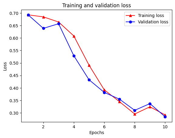
plt.plot(epochs, loss, '-r^', label='Training loss')
# "-b0" is for solid blue line with circle markers.
plt.plot(epochs, val_loss, '-bo', label='Validation loss')
plt.title('Training and validation loss')
plt.xlabel('Epochs')
plt.ylabel('Loss')
plt.legend(loc='best')
plt.show()
plt.clf() # clear figure
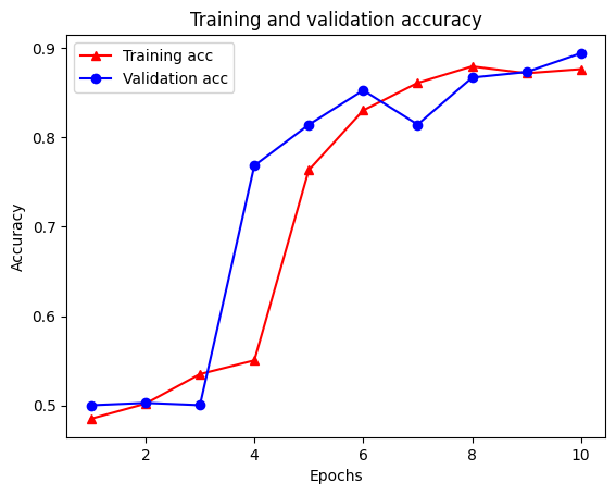
plt.plot(epochs, acc, '-r^', label='Training acc')
plt.plot(epochs, val_acc, '-bo', label='Validation acc')
plt.title('Training and validation accuracy')
plt.xlabel('Epochs')
plt.ylabel('Accuracy')
plt.legend(loc='best')
plt.show()
トレーニング損失は各エポック各エポックとトレーニング精度増加と共に減少に気づきます。これは、最急降下法の最適化を使用する場合に予想されます。反復ごとに必要な量を最小化する必要があります。
グラフの正則化
これで、上記で作成した基本モデルを使用してグラフの正則化を試す準備ができました。我々が使用するGraphRegularizationグラフ正則化を含むように塩基(双LSTM)モデルをラップするニューラル構造の学習フレームワークによって提供されるラッパークラスを。グラフ正則化モデルのトレーニングと評価の残りの手順は、基本モデルの手順と同様です。
グラフ正則化モデルを作成する
グラフの正則化の利点を評価するために、新しいベースモデルインスタンスを作成します。これは、あるmodelすでに数回の反復のために訓練されており、グラフ-正則モデルを作成するには、この訓練されたモデルを再利用するための公正な比較ではありませんmodel 。
# Build a new base LSTM model.
base_reg_model = make_bilstm_model()
# Wrap the base model with graph regularization.
graph_reg_config = nsl.configs.make_graph_reg_config(
    max_neighbors=HPARAMS.num_neighbors,
    multiplier=HPARAMS.graph_regularization_multiplier,
    distance_type=HPARAMS.distance_type,
    sum_over_axis=-1)
graph_reg_model = nsl.keras.GraphRegularization(base_reg_model,
                                                graph_reg_config)
graph_reg_model.compile(
    optimizer='adam',
    loss=tf.keras.losses.BinaryCrossentropy(from_logits=True),
    metrics=['accuracy'])
モデルをトレーニングする
graph_reg_history = graph_reg_model.fit(
    train_dataset,
    validation_data=validation_dataset,
    epochs=HPARAMS.train_epochs,
    verbose=1)
Epoch 1/10
/tmpfs/src/tf_docs_env/lib/python3.7/site-packages/tensorflow/python/framework/indexed_slices.py:446: UserWarning: Converting sparse IndexedSlices(IndexedSlices(indices=Tensor("gradient_tape/GraphRegularization/graph_loss/Reshape_1:0", shape=(None,), dtype=int32), values=Tensor("gradient_tape/GraphRegularization/graph_loss/Reshape:0", shape=(None, 1), dtype=float32), dense_shape=Tensor("gradient_tape/GraphRegularization/graph_loss/Cast:0", shape=(2,), dtype=int32))) to a dense Tensor of unknown shape. This may consume a large amount of memory.
  "shape. This may consume a large amount of memory." % value)
21/21 [==============================] - 28s 1s/step - loss: 0.6928 - accuracy: 0.5131 - scaled_graph_loss: 4.3840e-05 - val_loss: 0.6923 - val_accuracy: 0.4997
Epoch 2/10
21/21 [==============================] - 19s 939ms/step - loss: 0.6852 - accuracy: 0.5158 - scaled_graph_loss: 0.0021 - val_loss: 0.6818 - val_accuracy: 0.4996
Epoch 3/10
21/21 [==============================] - 19s 939ms/step - loss: 0.6698 - accuracy: 0.5123 - scaled_graph_loss: 0.0021 - val_loss: 0.6534 - val_accuracy: 0.5001
Epoch 4/10
21/21 [==============================] - 20s 959ms/step - loss: 0.6194 - accuracy: 0.6285 - scaled_graph_loss: 0.0284 - val_loss: 0.5297 - val_accuracy: 0.7955
Epoch 5/10
21/21 [==============================] - 19s 937ms/step - loss: 0.5805 - accuracy: 0.7346 - scaled_graph_loss: 0.0545 - val_loss: 0.5601 - val_accuracy: 0.6349
Epoch 6/10
21/21 [==============================] - 19s 934ms/step - loss: 0.5509 - accuracy: 0.7662 - scaled_graph_loss: 0.0654 - val_loss: 0.4899 - val_accuracy: 0.7538
Epoch 7/10
21/21 [==============================] - 19s 937ms/step - loss: 0.5326 - accuracy: 0.7877 - scaled_graph_loss: 0.0701 - val_loss: 0.4395 - val_accuracy: 0.7923
Epoch 8/10
21/21 [==============================] - 20s 940ms/step - loss: 0.5157 - accuracy: 0.8258 - scaled_graph_loss: 0.0811 - val_loss: 0.4585 - val_accuracy: 0.7909
Epoch 9/10
21/21 [==============================] - 19s 937ms/step - loss: 0.5063 - accuracy: 0.8388 - scaled_graph_loss: 0.0868 - val_loss: 0.4272 - val_accuracy: 0.8433
Epoch 10/10
21/21 [==============================] - 19s 934ms/step - loss: 0.5053 - accuracy: 0.8438 - scaled_graph_loss: 0.0858 - val_loss: 0.4485 - val_accuracy: 0.7680
モデルを評価する
graph_reg_results = graph_reg_model.evaluate(test_dataset, steps=HPARAMS.eval_steps)
print(graph_reg_results)
196/196 [==============================] - 16s 76ms/step - loss: 0.4890 - accuracy: 0.7246
[0.4889770448207855, 0.7246000170707703]
時間の経過に伴う精度/損失のグラフを作成します
graph_reg_history_dict = graph_reg_history.history
graph_reg_history_dict.keys()
dict_keys(['loss', 'accuracy', 'scaled_graph_loss', 'val_loss', 'val_accuracy'])
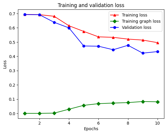
ディクショナリには、トレーニング損失、トレーニング精度、トレーニンググラフ損失、検証損失、および検証精度の合計5つのエントリがあります。比較のためにそれらをすべて一緒にプロットできます。グラフの損失はトレーニング中にのみ計算されることに注意してください。
acc = graph_reg_history_dict['accuracy']
val_acc = graph_reg_history_dict['val_accuracy']
loss = graph_reg_history_dict['loss']
graph_loss = graph_reg_history_dict['scaled_graph_loss']
val_loss = graph_reg_history_dict['val_loss']

epochs = range(1, len(acc) + 1)

plt.clf()   # clear figure

# "-r^" is for solid red line with triangle markers.
plt.plot(epochs, loss, '-r^', label='Training loss')
# "-gD" is for solid green line with diamond markers.
plt.plot(epochs, graph_loss, '-gD', label='Training graph loss')
# "-b0" is for solid blue line with circle markers.
plt.plot(epochs, val_loss, '-bo', label='Validation loss')
plt.title('Training and validation loss')
plt.xlabel('Epochs')
plt.ylabel('Loss')
plt.legend(loc='best')

plt.show()
plt.clf() # clear figure
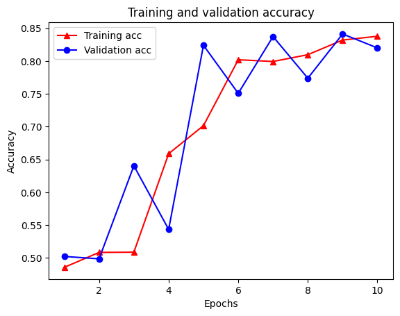
plt.plot(epochs, acc, '-r^', label='Training acc')
plt.plot(epochs, val_acc, '-bo', label='Validation acc')
plt.title('Training and validation accuracy')
plt.xlabel('Epochs')
plt.ylabel('Accuracy')
plt.legend(loc='best')
plt.show()
半教師あり学習の力
半教師あり学習、より具体的には、このチュートリアルのコンテキストでのグラフの正則化は、トレーニングデータの量が少ない場合に非常に強力になります。トレーニングデータの不足は、トレーニングサンプル間の類似性を活用することで補われます。これは、従来の教師あり学習では不可能です。
我々は、トレーニング、検証、試験サンプルを含むサンプルの総数に対する訓練サンプルの比として監督の比を規定します。このノートブックでは、基本モデルとグラフ正則化モデルの両方をトレーニングするために、0.05の監視率(つまり、ラベル付けされたデータの5%)を使用しました。以下のセルで、監視比率がモデルの精度に与える影響を示します。
# Accuracy values for both the Bi-LSTM model and the feed forward NN model have
# been precomputed for the following supervision ratios.

supervision_ratios = [0.3, 0.15, 0.05, 0.03, 0.02, 0.01, 0.005]

model_tags = ['Bi-LSTM model', 'Feed Forward NN model']
base_model_accs = [[84, 84, 83, 80, 65, 52, 50], [87, 86, 76, 74, 67, 52, 51]]
graph_reg_model_accs = [[84, 84, 83, 83, 65, 63, 50],
                        [87, 86, 80, 75, 67, 52, 50]]

plt.clf()  # clear figure

fig, axes = plt.subplots(1, 2)
fig.set_size_inches((12, 5))

for ax, model_tag, base_model_acc, graph_reg_model_acc in zip(
    axes, model_tags, base_model_accs, graph_reg_model_accs):

  # "-r^" is for solid red line with triangle markers.
  ax.plot(base_model_acc, '-r^', label='Base model')
  # "-gD" is for solid green line with diamond markers.
  ax.plot(graph_reg_model_acc, '-gD', label='Graph-regularized model')
  ax.set_title(model_tag)
  ax.set_xlabel('Supervision ratio')
  ax.set_ylabel('Accuracy(%)')
  ax.set_ylim((25, 100))
  ax.set_xticks(range(len(supervision_ratios)))
  ax.set_xticklabels(supervision_ratios)
  ax.legend(loc='best')

plt.show()
<Figure size 432x288 with 0 Axes>
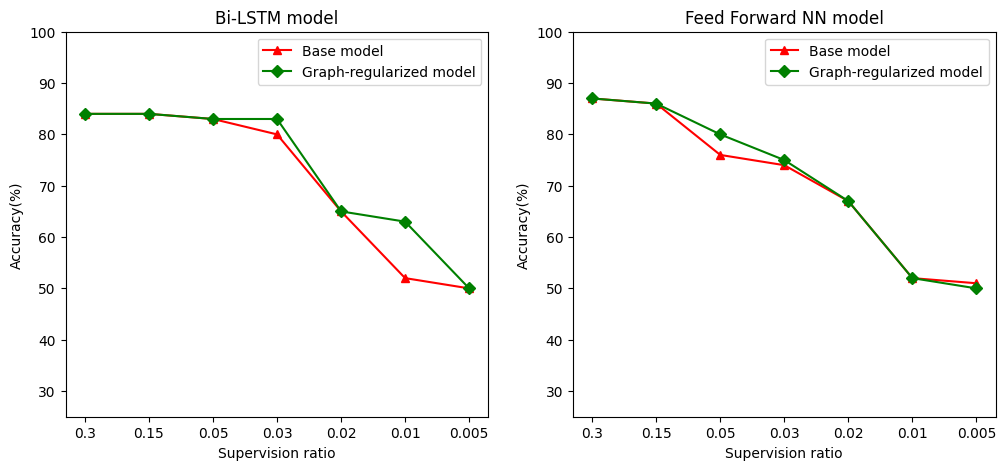
監視率が低下すると、モデルの精度も低下することがわかります。これは、使用されるモデルアーキテクチャに関係なく、基本モデルとグラフ正則化モデルの両方に当てはまります。ただし、グラフで正則化されたモデルは、両方のアーキテクチャの基本モデルよりもパフォーマンスが優れていることに注意してください。監督比が0.01である場合、特に、バイLSTMモデルのために、グラフ正規モデルの精度は、20%より高いベースモデルに比べ〜あります。これは主に、トレーニングサンプル自体に加えてトレーニングサンプル間の構造的類似性が使用される、グラフ正則化モデルの半教師あり学習によるものです。
結論
入力に明示的なグラフが含まれていない場合でも、Neural Structured Learning(NSL)フレームワークを使用したグラフ正則化の使用を示しました。レビューの埋め込みに基づいて類似性グラフを合成したIMDB映画レビューの感情分類のタスクを検討しました。ハイパーパラメータや監視の量を変えたり、さまざまなモデルアーキテクチャを使用したりして、さらに実験することをお勧めします。