|
|
|
 View source on GitHub View source on GitHub
|
|
This tutorial builds a quantum neural network (QNN) to classify a simplified version of MNIST, similar to the approach used in Farhi et al. The performance of the quantum neural network on this classical data problem is compared with a classical neural network.
Setup
Install TensorFlow and TensorFlow Quantum:
# In Colab, you will be asked to restart the session after this finishes.pip install tensorflow==2.18.1 tensorflow-quantum==0.7.6
# Install seaborn for use later in this notebook.pip install seaborn
Configure the use of Keras 2:
import os

# Keras 2 must be selected before importing TensorFlow or TensorFlow Quantum:
os.environ["TF_USE_LEGACY_KERAS"] = "1"
Now import TensorFlow, TensorFlow Quantum, and other modules needed:
import tensorflow as tf
import tensorflow_quantum as tfq

import cirq
import sympy
import numpy as np
import seaborn as sns
import collections

# visualization tools
%matplotlib inline
import matplotlib.pyplot as plt
from cirq.contrib.svg import SVGCircuit
2026-04-18 07:52:37.284737: E external/local_xla/xla/stream_executor/cuda/cuda_fft.cc:477] Unable to register cuFFT factory: Attempting to register factory for plugin cuFFT when one has already been registered
WARNING: All log messages before absl::InitializeLog() is called are written to STDERR
E0000 00:00:1776513157.306740   22046 cuda_dnn.cc:8310] Unable to register cuDNN factory: Attempting to register factory for plugin cuDNN when one has already been registered
E0000 00:00:1776513157.313538   22046 cuda_blas.cc:1418] Unable to register cuBLAS factory: Attempting to register factory for plugin cuBLAS when one has already been registered
2026-04-18 07:52:41.686430: E external/local_xla/xla/stream_executor/cuda/cuda_driver.cc:152] failed call to cuInit: INTERNAL: CUDA error: Failed call to cuInit: CUDA_ERROR_NO_DEVICE: no CUDA-capable device is detected
1. Load the data
In this tutorial you will build a binary classifier to distinguish between the digits 3 and 6, following Farhi et al. This section covers the data handling that:
- Loads the raw data from Keras.
- Filters the dataset to only 3s and 6s.
- Downscales the images so they can fit in a quantum computer.
- Removes any contradictory examples.
- Converts the binary images to Cirq circuits.
- Converts the Cirq circuits to TensorFlow Quantum circuits.
1.1 Load the raw data
Load the MNIST dataset distributed with Keras.
(x_train, y_train), (x_test, y_test) = tf.keras.datasets.mnist.load_data()

# Rescale the images from [0,255] to the [0.0,1.0] range.
x_train, x_test = x_train[..., np.newaxis] / 255.0, x_test[...,
                                                           np.newaxis] / 255.0

print("Number of original training examples:", len(x_train))
print("Number of original test examples:", len(x_test))
Downloading data from https://storage.googleapis.com/tensorflow/tf-keras-datasets/mnist.npz
11490434/11490434 [==============================] - 0s 0us/step
Number of original training examples: 60000
Number of original test examples: 10000
Filter the dataset to keep just the 3s and 6s, remove the other classes. At the same time convert the label, y, to boolean: True for 3 and False for 6.
def filter_36(x, y):
    keep = (y == 3) | (y == 6)
    x, y = x[keep], y[keep]
    y = y == 3
    return x, y
x_train, y_train = filter_36(x_train, y_train)
x_test, y_test = filter_36(x_test, y_test)

print("Number of filtered training examples:", len(x_train))
print("Number of filtered test examples:", len(x_test))
Number of filtered training examples: 12049
Number of filtered test examples: 1968
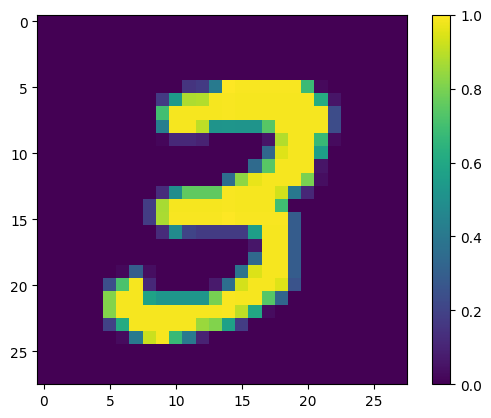
Show the first example:
print(y_train[0])

plt.imshow(x_train[0, :, :, 0])
plt.colorbar()
True
<matplotlib.colorbar.Colorbar at 0x7faec2797610>
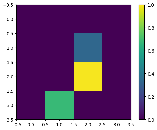
1.2 Downscale the images
An image size of 28x28 is much too large for current quantum computers. Resize the image down to 4x4:
x_train_small = tf.image.resize(x_train, (4, 4)).numpy()
x_test_small = tf.image.resize(x_test, (4, 4)).numpy()
Again, display the first training example—after resize:
print(y_train[0])

plt.imshow(x_train_small[0, :, :, 0], vmin=0, vmax=1)
plt.colorbar()
True
<matplotlib.colorbar.Colorbar at 0x7faec2717cd0>
1.3 Remove contradictory examples
From section 3.3 Learning to Distinguish Digits of Farhi et al., filter the dataset to remove images that are labeled as belonging to both classes.
This is not a standard machine-learning procedure, but is included in the interest of following the paper.
def remove_contradicting(xs, ys):
    mapping = collections.defaultdict(set)
    orig_x = {}
    # Determine the set of labels for each unique image:
    for x, y in zip(xs, ys):
        orig_x[tuple(x.flatten())] = x
        mapping[tuple(x.flatten())].add(y)

    new_x = []
    new_y = []
    for flatten_x in mapping:
        x = orig_x[flatten_x]
        labels = mapping[flatten_x]
        if len(labels) == 1:
            new_x.append(x)
            new_y.append(next(iter(labels)))
        else:
            # Throw out images that match more than one label.
            pass

    num_uniq_3 = sum(
        1 for value in mapping.values() if len(value) == 1 and True in value)
    num_uniq_6 = sum(
        1 for value in mapping.values() if len(value) == 1 and False in value)
    num_uniq_both = sum(1 for value in mapping.values() if len(value) == 2)

    print("Number of unique images:", len(mapping.values()))
    print("Number of unique 3s: ", num_uniq_3)
    print("Number of unique 6s: ", num_uniq_6)
    print("Number of unique contradicting labels (both 3 and 6): ",
          num_uniq_both)
    print()
    print("Initial number of images: ", len(xs))
    print("Remaining non-contradicting unique images: ", len(new_x))

    return np.array(new_x), np.array(new_y)
The resulting counts do not closely match the reported values, but the exact procedure is not specified.
It is also worth noting here that applying filtering contradictory examples at this point does not totally prevent the model from receiving contradictory training examples: the next step binarizes the data which will cause more collisions.
x_train_nocon, y_train_nocon = remove_contradicting(x_train_small, y_train)
Number of unique images: 10387
Number of unique 3s:  4912
Number of unique 6s:  5426
Number of unique contradicting labels (both 3 and 6):  49

Initial number of images:  12049
Remaining non-contradicting unique images:  10338
1.4 Encode the data as quantum circuits
To process images using a quantum computer, Farhi et al. proposed representing each pixel with a qubit, with the state depending on the value of the pixel. The first step is to convert to a binary encoding.
THRESHOLD = 0.5

x_train_bin = np.array(x_train_nocon > THRESHOLD, dtype=np.float32)
x_test_bin = np.array(x_test_small > THRESHOLD, dtype=np.float32)
If you were to remove contradictory images at this point you would be left with only 193, likely not enough for effective training.
_ = remove_contradicting(x_train_bin, y_train_nocon)
Number of unique images: 193
Number of unique 3s:  80
Number of unique 6s:  69
Number of unique contradicting labels (both 3 and 6):  44

Initial number of images:  10338
Remaining non-contradicting unique images:  149
The qubits at pixel indices with values that exceed a threshold, are rotated through an \(X\) gate.
def convert_to_circuit(image):
    """Encode truncated classical image into quantum datapoint."""
    values = np.ndarray.flatten(image)
    qubits = cirq.GridQubit.rect(4, 4)
    circuit = cirq.Circuit()
    for i, value in enumerate(values):
        if value:
            circuit.append(cirq.X(qubits[i]))
    return circuit


x_train_circ = [convert_to_circuit(x) for x in x_train_bin]
x_test_circ = [convert_to_circuit(x) for x in x_test_bin]
Here is the circuit created for the first example (circuit diagrams do not show qubits with zero gates):
SVGCircuit(x_train_circ[0])

Compare this circuit to the indices where the image value exceeds the threshold:
bin_img = x_train_bin[0, :, :, 0]
indices = np.array(np.where(bin_img)).T
indices
array([[2, 2],
       [3, 1]])
Convert these Cirq circuits to tensors for tfq:
x_train_tfcirc = tfq.convert_to_tensor(x_train_circ)
x_test_tfcirc = tfq.convert_to_tensor(x_test_circ)
2. Quantum neural network
There is little guidance for a quantum circuit structure that classifies images. Since the classification is based on the expectation of the readout qubit, Farhi et al. propose using two qubit gates, with the readout qubit always acted upon. This is similar in some ways to running small a Unitary RNN across the pixels.
2.1 Build the model circuit
This following example shows this layered approach. Each layer uses n instances of the same gate, with each of the data qubits acting on the readout qubit.
Start with a simple class that will add a layer of these gates to a circuit:
class CircuitLayerBuilder():

    def __init__(self, data_qubits, readout):
        self.data_qubits = data_qubits
        self.readout = readout

    def add_layer(self, circuit, gate, prefix):
        for i, qubit in enumerate(self.data_qubits):
            symbol = sympy.Symbol(prefix + '-' + str(i))
            circuit.append(gate(qubit, self.readout)**symbol)
Build an example circuit layer to see how it looks:
demo_builder = CircuitLayerBuilder(data_qubits=cirq.GridQubit.rect(4, 1),
                                   readout=cirq.GridQubit(-1, -1))

circuit = cirq.Circuit()
demo_builder.add_layer(circuit, gate=cirq.XX, prefix='xx')
SVGCircuit(circuit)

Now build a two-layered model, matching the data-circuit size, and include the preparation and readout operations.
def create_quantum_model():
    """Create a QNN model circuit and readout operation to go along with it."""
    data_qubits = cirq.GridQubit.rect(4, 4)  # a 4x4 grid.
    readout = cirq.GridQubit(-1, -1)  # a single qubit at [-1,-1]
    circuit = cirq.Circuit()

    # Prepare the readout qubit.
    circuit.append(cirq.X(readout))
    circuit.append(cirq.H(readout))

    builder = CircuitLayerBuilder(data_qubits=data_qubits, readout=readout)

    # Then add layers (experiment by adding more).
    builder.add_layer(circuit, cirq.XX, "xx1")
    builder.add_layer(circuit, cirq.ZZ, "zz1")

    # Finally, prepare the readout qubit.
    circuit.append(cirq.H(readout))

    return circuit, cirq.Z(readout)
model_circuit, model_readout = create_quantum_model()
2.2 Wrap the model-circuit in a tfq-keras model
Build the Keras model with the quantum components. This model is fed the "quantum data", from x_train_circ, that encodes the classical data. It uses a Parametrized Quantum Circuit layer, tfq.layers.PQC, to train the model circuit, on the quantum data.
To classify these images, Farhi et al. proposed taking the expectation of a readout qubit in a parameterized circuit. The expectation returns a value between 1 and -1.
# Build the Keras model.
model = tf.keras.Sequential([
    # The input is the data-circuit, encoded as a tf.string
    tf.keras.layers.Input(shape=(), dtype=tf.string),
    # The PQC layer returns the expected value of the readout gate, range [-1,1].
    tfq.layers.PQC(model_circuit, model_readout),
])
Next, describe the training procedure to the model, using the compile method.
Since the expected readout is in the range [-1,1], optimizing the hinge loss is a somewhat natural fit.
To use the hinge loss here you need to make two small adjustments. First convert the labels, y_train_nocon, from boolean to [-1,1], as expected by the hinge loss.
y_train_hinge = 2.0 * y_train_nocon - 1.0
y_test_hinge = 2.0 * y_test - 1.0
Second, use a custom hinge_accuracy metric that correctly handles [-1, 1] as the y_true labels argument.
tf.losses.BinaryAccuracy(threshold=0.0) expects y_true to be a boolean, and so can't be used with hinge loss).
def hinge_accuracy(y_true, y_pred):
    y_true = tf.squeeze(y_true) > 0.0
    y_pred = tf.squeeze(y_pred) > 0.0
    result = tf.cast(y_true == y_pred, tf.float32)

    return tf.reduce_mean(result)
model.compile(loss=tf.keras.losses.Hinge(),
              optimizer=tf.keras.optimizers.Adam(),
              metrics=[hinge_accuracy])
print(model.summary())
Model: "sequential"
_________________________________________________________________
 Layer (type)                Output Shape              Param #
=================================================================
 pqc (PQC)                   (None, 1)                 32

=================================================================
Total params: 32 (128.00 Byte)
Trainable params: 32 (128.00 Byte)
Non-trainable params: 0 (0.00 Byte)
_________________________________________________________________
None
Train the quantum model
Now train the model—this takes about 45 min. If you don't want to wait that long, use a small subset of the data (set NUM_EXAMPLES=500, below). This doesn't really affect the model's progress during training (it only has 32 parameters, and doesn't need much data to constrain these). Using fewer examples just ends training earlier (5min), but runs long enough to show that it is making progress in the validation logs.
EPOCHS = 3
BATCH_SIZE = 32

NUM_EXAMPLES = len(x_train_tfcirc)
x_train_tfcirc_sub = x_train_tfcirc[:NUM_EXAMPLES]
y_train_hinge_sub = y_train_hinge[:NUM_EXAMPLES]
Training this model to convergence should achieve >85% accuracy on the test set.
qnn_history = model.fit(x_train_tfcirc_sub,
                        y_train_hinge_sub,
                        batch_size=BATCH_SIZE,
                        epochs=EPOCHS,
                        verbose=1,
                        validation_data=(x_test_tfcirc, y_test_hinge))

qnn_results = model.evaluate(x_test_tfcirc, y_test)
Epoch 1/3
324/324 [==============================] - 212s 653ms/step - loss: 0.6775 - hinge_accuracy: 0.7638 - val_loss: 0.4140 - val_hinge_accuracy: 0.8080
Epoch 2/3
324/324 [==============================] - 211s 651ms/step - loss: 0.3887 - hinge_accuracy: 0.8474 - val_loss: 0.3640 - val_hinge_accuracy: 0.8816
Epoch 3/3
324/324 [==============================] - 211s 650ms/step - loss: 0.3698 - hinge_accuracy: 0.8628 - val_loss: 0.3455 - val_hinge_accuracy: 0.8977
62/62 [==============================] - 7s 114ms/step - loss: 0.3455 - hinge_accuracy: 0.8977
3. Classical neural network
While the quantum neural network works for this simplified MNIST problem, a basic classical neural network can easily outperform a QNN on this task. After a single epoch, a classical neural network can achieve >98% accuracy on the holdout set.
In the following example, a classical neural network is used for for the 3-6 classification problem using the entire 28x28 image instead of subsampling the image. This easily converges to nearly 100% accuracy of the test set.
def create_classical_model():
    # A simple model based off LeNet from https://keras.io/examples/mnist_cnn/
    model = tf.keras.Sequential()
    model.add(
        tf.keras.layers.Conv2D(32, [3, 3],
                               activation='relu',
                               input_shape=(28, 28, 1)))
    model.add(tf.keras.layers.Conv2D(64, [3, 3], activation='relu'))
    model.add(tf.keras.layers.MaxPooling2D(pool_size=(2, 2)))
    model.add(tf.keras.layers.Dropout(0.25))
    model.add(tf.keras.layers.Flatten())
    model.add(tf.keras.layers.Dense(128, activation='relu'))
    model.add(tf.keras.layers.Dropout(0.5))
    model.add(tf.keras.layers.Dense(1))
    return model


model = create_classical_model()
model.compile(loss=tf.keras.losses.BinaryCrossentropy(from_logits=True),
              optimizer=tf.keras.optimizers.Adam(),
              metrics=['accuracy'])

model.summary()
Model: "sequential_1"
_________________________________________________________________
 Layer (type)                Output Shape              Param #
=================================================================
 conv2d (Conv2D)             (None, 26, 26, 32)        320

 conv2d_1 (Conv2D)           (None, 24, 24, 64)        18496

 max_pooling2d (MaxPooling2  (None, 12, 12, 64)        0
 D)

 dropout (Dropout)           (None, 12, 12, 64)        0

 flatten (Flatten)           (None, 9216)              0

 dense (Dense)               (None, 128)               1179776

 dropout_1 (Dropout)         (None, 128)               0

 dense_1 (Dense)             (None, 1)                 129

=================================================================
Total params: 1198721 (4.57 MB)
Trainable params: 1198721 (4.57 MB)
Non-trainable params: 0 (0.00 Byte)
_________________________________________________________________
model.fit(x_train,
          y_train,
          batch_size=128,
          epochs=1,
          verbose=1,
          validation_data=(x_test, y_test))

cnn_results = model.evaluate(x_test, y_test)
95/95 [==============================] - 12s 122ms/step - loss: 0.0433 - accuracy: 0.9841 - val_loss: 0.0028 - val_accuracy: 0.9995
62/62 [==============================] - 1s 9ms/step - loss: 0.0028 - accuracy: 0.9995
The above model has nearly 1.2M parameters. For a more fair comparison, try a 37-parameter model, on the subsampled images:
def create_fair_classical_model():
    # A simple model based off LeNet from https://keras.io/examples/mnist_cnn/
    model = tf.keras.Sequential()
    model.add(tf.keras.layers.Flatten(input_shape=(4, 4, 1)))
    model.add(tf.keras.layers.Dense(2, activation='relu'))
    model.add(tf.keras.layers.Dense(1))
    return model


model = create_fair_classical_model()
model.compile(loss=tf.keras.losses.BinaryCrossentropy(from_logits=True),
              optimizer=tf.keras.optimizers.Adam(),
              metrics=['accuracy'])

model.summary()
Model: "sequential_2"
_________________________________________________________________
 Layer (type)                Output Shape              Param #
=================================================================
 flatten_1 (Flatten)         (None, 16)                0

 dense_2 (Dense)             (None, 2)                 34

 dense_3 (Dense)             (None, 1)                 3

=================================================================
Total params: 37 (148.00 Byte)
Trainable params: 37 (148.00 Byte)
Non-trainable params: 0 (0.00 Byte)
_________________________________________________________________
model.fit(x_train_bin,
          y_train_nocon,
          batch_size=128,
          epochs=20,
          verbose=2,
          validation_data=(x_test_bin, y_test))

fair_nn_results = model.evaluate(x_test_bin, y_test)
Epoch 1/20
81/81 - 1s - loss: 0.6125 - accuracy: 0.5249 - val_loss: 0.6129 - val_accuracy: 0.4868 - 732ms/epoch - 9ms/step
Epoch 2/20
81/81 - 0s - loss: 0.5737 - accuracy: 0.5249 - val_loss: 0.5730 - val_accuracy: 0.4868 - 136ms/epoch - 2ms/step
Epoch 3/20
81/81 - 0s - loss: 0.5269 - accuracy: 0.5270 - val_loss: 0.5139 - val_accuracy: 0.5000 - 140ms/epoch - 2ms/step
Epoch 4/20
81/81 - 0s - loss: 0.4624 - accuracy: 0.6776 - val_loss: 0.4429 - val_accuracy: 0.8135 - 138ms/epoch - 2ms/step
Epoch 5/20
81/81 - 0s - loss: 0.3999 - accuracy: 0.8380 - val_loss: 0.3826 - val_accuracy: 0.8267 - 137ms/epoch - 2ms/step
Epoch 6/20
81/81 - 0s - loss: 0.3507 - accuracy: 0.8448 - val_loss: 0.3380 - val_accuracy: 0.8267 - 139ms/epoch - 2ms/step
Epoch 7/20
81/81 - 0s - loss: 0.3152 - accuracy: 0.8455 - val_loss: 0.3063 - val_accuracy: 0.8267 - 143ms/epoch - 2ms/step
Epoch 8/20
81/81 - 0s - loss: 0.2900 - accuracy: 0.8463 - val_loss: 0.2835 - val_accuracy: 0.8267 - 147ms/epoch - 2ms/step
Epoch 9/20
81/81 - 0s - loss: 0.2719 - accuracy: 0.8624 - val_loss: 0.2666 - val_accuracy: 0.8653 - 141ms/epoch - 2ms/step
Epoch 10/20
81/81 - 0s - loss: 0.2588 - accuracy: 0.8693 - val_loss: 0.2547 - val_accuracy: 0.8664 - 138ms/epoch - 2ms/step
Epoch 11/20
81/81 - 0s - loss: 0.2494 - accuracy: 0.8717 - val_loss: 0.2455 - val_accuracy: 0.8664 - 136ms/epoch - 2ms/step
Epoch 12/20
81/81 - 0s - loss: 0.2422 - accuracy: 0.8744 - val_loss: 0.2391 - val_accuracy: 0.8669 - 138ms/epoch - 2ms/step
Epoch 13/20
81/81 - 0s - loss: 0.2370 - accuracy: 0.8762 - val_loss: 0.2342 - val_accuracy: 0.8674 - 138ms/epoch - 2ms/step
Epoch 14/20
81/81 - 0s - loss: 0.2330 - accuracy: 0.8769 - val_loss: 0.2303 - val_accuracy: 0.8674 - 136ms/epoch - 2ms/step
Epoch 15/20
81/81 - 0s - loss: 0.2299 - accuracy: 0.8771 - val_loss: 0.2274 - val_accuracy: 0.8679 - 138ms/epoch - 2ms/step
Epoch 16/20
81/81 - 0s - loss: 0.2275 - accuracy: 0.8788 - val_loss: 0.2251 - val_accuracy: 0.8689 - 138ms/epoch - 2ms/step
Epoch 17/20
81/81 - 0s - loss: 0.2256 - accuracy: 0.8805 - val_loss: 0.2233 - val_accuracy: 0.8689 - 138ms/epoch - 2ms/step
Epoch 18/20
81/81 - 0s - loss: 0.2242 - accuracy: 0.8822 - val_loss: 0.2221 - val_accuracy: 0.8689 - 142ms/epoch - 2ms/step
Epoch 19/20
81/81 - 0s - loss: 0.2231 - accuracy: 0.8968 - val_loss: 0.2210 - val_accuracy: 0.9157 - 139ms/epoch - 2ms/step
Epoch 20/20
81/81 - 0s - loss: 0.2221 - accuracy: 0.9039 - val_loss: 0.2200 - val_accuracy: 0.9162 - 137ms/epoch - 2ms/step
62/62 [==============================] - 0s 1ms/step - loss: 0.2200 - accuracy: 0.9162
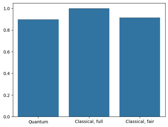
4. Comparison
Higher resolution input and a more powerful model make this problem easy for the CNN. While a classical model of similar power (~32 parameters) trains to a similar accuracy in a fraction of the time. One way or the other, the classical neural network easily outperforms the quantum neural network. For classical data, it is difficult to beat a classical neural network.
qnn_accuracy = qnn_results[1]
cnn_accuracy = cnn_results[1]
fair_nn_accuracy = fair_nn_results[1]

sns.barplot(x=["Quantum", "Classical, full", "Classical, fair"],
            y=[qnn_accuracy, cnn_accuracy, fair_nn_accuracy])
<Axes: >