
| | |  Ver fuente en GitHub Ver fuente en GitHub |
Este cuaderno forma a una secuencia a secuencia modelo (seq2seq) para la traducción del español al Inglés basado en enfoques eficaces para la traducción automática neuronal basada en la atención . Este es un ejemplo avanzado que asume cierto conocimiento de:
- Secuencia a secuenciar modelos
- Fundamentos de TensorFlow debajo de la capa de keras:
- Trabajar con tensores directamente
- Personalizado escrito
keras.Models ykeras.layers
Mientras que esta arquitectura no está actualizado un poco todavía es un proyecto de gran utilidad para el trabajo a través de obtener una comprensión más profunda de los mecanismos de atención (antes de pasar a los transformadores ).
Después de entrenar el modelo en este cuaderno, usted será capaz de introducir una sentencia española, como por ejemplo, y devolver la traducción en Inglés "¿todavia estan en casa?": "¿Está usted todavía en casa"
El modelo resultante es exportable como tf.saved_model , por lo que puede ser utilizado en otros entornos TensorFlow.
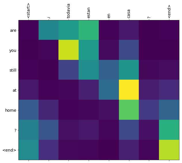
La calidad de la traducción es razonable para un ejemplo de juguete, pero la trama de atención generada es quizás más interesante. Esto muestra qué partes de la oración de entrada llaman la atención del modelo mientras traduce:
Configuración
pip install tensorflow_text
import numpy as np

import typing
from typing import Any, Tuple

import tensorflow as tf

import tensorflow_text as tf_text

import matplotlib.pyplot as plt
import matplotlib.ticker as ticker
Este tutorial crea algunas capas desde cero, use esta variable si desea cambiar entre las implementaciones personalizadas e integradas.
use_builtins = True
Este tutorial utiliza muchas API de bajo nivel en las que es fácil equivocar las formas. Esta clase se usa para verificar formas a lo largo del tutorial.
Comprobador de forma
class ShapeChecker():
  def __init__(self):
    # Keep a cache of every axis-name seen
    self.shapes = {}

  def __call__(self, tensor, names, broadcast=False):
    if not tf.executing_eagerly():
      return

    if isinstance(names, str):
      names = (names,)

    shape = tf.shape(tensor)
    rank = tf.rank(tensor)

    if rank != len(names):
      raise ValueError(f'Rank mismatch:\n'
                       f'    found {rank}: {shape.numpy()}\n'
                       f'    expected {len(names)}: {names}\n')

    for i, name in enumerate(names):
      if isinstance(name, int):
        old_dim = name
      else:
        old_dim = self.shapes.get(name, None)
      new_dim = shape[i]

      if (broadcast and new_dim == 1):
        continue

      if old_dim is None:
        # If the axis name is new, add its length to the cache.
        self.shapes[name] = new_dim
        continue

      if new_dim != old_dim:
        raise ValueError(f"Shape mismatch for dimension: '{name}'\n"
                         f"    found: {new_dim}\n"
                         f"    expected: {old_dim}\n")
Los datos
Vamos a utilizar un conjunto de datos proporcionado por el lenguaje http://www.manythings.org/anki/ Este conjunto de datos contiene pares de traducción de idiomas en el formato:
May I borrow this book? ¿Puedo tomar prestado este libro?
Tienen una variedad de idiomas disponibles, pero usaremos el conjunto de datos inglés-español.
Descarga y prepara el conjunto de datos
Para su comodidad, hemos alojado una copia de este conjunto de datos en Google Cloud, pero también puede descargar su propia copia. Después de descargar el conjunto de datos, estos son los pasos que seguiremos para preparar los datos:
- Añadir un nuevo comienzo y al final de contadores a cada frase.
- Limpia las oraciones eliminando caracteres especiales.
- Cree un índice de palabras y un índice de palabras inverso (asignación de diccionarios de palabra → id e id → palabra).
- Rellena cada oración a una longitud máxima.
# Download the file
import pathlib

path_to_zip = tf.keras.utils.get_file(
    'spa-eng.zip', origin='http://storage.googleapis.com/download.tensorflow.org/data/spa-eng.zip',
    extract=True)

path_to_file = pathlib.Path(path_to_zip).parent/'spa-eng/spa.txt'
Downloading data from http://storage.googleapis.com/download.tensorflow.org/data/spa-eng.zip
2646016/2638744 [==============================] - 0s 0us/step
2654208/2638744 [==============================] - 0s 0us/step
def load_data(path):
  text = path.read_text(encoding='utf-8')

  lines = text.splitlines()
  pairs = [line.split('\t') for line in lines]

  inp = [inp for targ, inp in pairs]
  targ = [targ for targ, inp in pairs]

  return targ, inp
targ, inp = load_data(path_to_file)
print(inp[-1])
Si quieres sonar como un hablante nativo, debes estar dispuesto a practicar diciendo la misma frase una y otra vez de la misma manera en que un músico de banjo practica el mismo fraseo una y otra vez hasta que lo puedan tocar correctamente y en el tiempo esperado.
print(targ[-1])
If you want to sound like a native speaker, you must be willing to practice saying the same sentence over and over in the same way that banjo players practice the same phrase over and over until they can play it correctly and at the desired tempo.
Crea un conjunto de datos tf.data
A partir de estas matrices de cadenas se puede crear un tf.data.Dataset de cadenas que baraja y lotes de manera eficiente:
BUFFER_SIZE = len(inp)
BATCH_SIZE = 64

dataset = tf.data.Dataset.from_tensor_slices((inp, targ)).shuffle(BUFFER_SIZE)
dataset = dataset.batch(BATCH_SIZE)
for example_input_batch, example_target_batch in dataset.take(1):
  print(example_input_batch[:5])
  print()
  print(example_target_batch[:5])
  break
tf.Tensor(
[b'No s\xc3\xa9 lo que quiero.' b'\xc2\xbfDeber\xc3\xada repetirlo?'
 b'Tard\xc3\xa9 m\xc3\xa1s de 2 horas en traducir unas p\xc3\xa1ginas en ingl\xc3\xa9s.'
 b'A Tom comenz\xc3\xb3 a temerle a Mary.' b'Mi pasatiempo es la lectura.'], shape=(5,), dtype=string)

tf.Tensor(
[b"I don't know what I want." b'Should I repeat it?'
 b'It took me more than two hours to translate a few pages of English.'
 b'Tom became afraid of Mary.' b'My hobby is reading.'], shape=(5,), dtype=string)
Preprocesamiento de texto
Uno de los objetivos de este tutorial es construir un modelo que puede ser exportado como un tf.saved_model . Para hacer que el modelo exportado útil que debe tomar tf.string entradas, y volver tf.string salidas: Todo el procesamiento de texto que ocurre dentro del modelo.
Estandarización
El modelo trata con texto multilingüe con un vocabulario limitado. Por eso será importante estandarizar el texto de entrada.
El primer paso es la normalización Unicode para dividir los caracteres acentuados y reemplazar los caracteres de compatibilidad con sus equivalentes ASCII.
El tensorflow_text paquete contiene una operación de normalizar Unicode:
example_text = tf.constant('¿Todavía está en casa?')

print(example_text.numpy())
print(tf_text.normalize_utf8(example_text, 'NFKD').numpy())
b'\xc2\xbfTodav\xc3\xada est\xc3\xa1 en casa?'
b'\xc2\xbfTodavi\xcc\x81a esta\xcc\x81 en casa?'
La normalización Unicode será el primer paso en la función de estandarización de texto:
def tf_lower_and_split_punct(text):
  # Split accecented characters.
  text = tf_text.normalize_utf8(text, 'NFKD')
  text = tf.strings.lower(text)
  # Keep space, a to z, and select punctuation.
  text = tf.strings.regex_replace(text, '[^ a-z.?!,¿]', '')
  # Add spaces around punctuation.
  text = tf.strings.regex_replace(text, '[.?!,¿]', r' \0 ')
  # Strip whitespace.
  text = tf.strings.strip(text)

  text = tf.strings.join(['[START]', text, '[END]'], separator=' ')
  return text
print(example_text.numpy().decode())
print(tf_lower_and_split_punct(example_text).numpy().decode())
¿Todavía está en casa?
[START] ¿ todavia esta en casa ? [END]
Vectorización de texto
Esta función de normalización será envuelto en una tf.keras.layers.TextVectorization capa que se encargará de la extracción vocabulario y la conversión de texto de entrada a las secuencias de tokens.
max_vocab_size = 5000

input_text_processor = tf.keras.layers.TextVectorization(
    standardize=tf_lower_and_split_punct,
    max_tokens=max_vocab_size)
El TextVectorization capa y muchas otras capas de preprocesamiento tienen una adapt método. Este método lee una época de los datos de entrenamiento, y funciona muy parecido a Model.fix . Este adapt método inicializa la capa a base de los datos. Aquí determina el vocabulario:
input_text_processor.adapt(inp)

# Here are the first 10 words from the vocabulary:
input_text_processor.get_vocabulary()[:10]
['', '[UNK]', '[START]', '[END]', '.', 'que', 'de', 'el', 'a', 'no']
Ese es el español TextVectorization capa, ahora construir y .adapt() del Inglés uno:
output_text_processor = tf.keras.layers.TextVectorization(
    standardize=tf_lower_and_split_punct,
    max_tokens=max_vocab_size)

output_text_processor.adapt(targ)
output_text_processor.get_vocabulary()[:10]
['', '[UNK]', '[START]', '[END]', '.', 'the', 'i', 'to', 'you', 'tom']
Ahora, estas capas pueden convertir un lote de cadenas en un lote de ID de token:
example_tokens = input_text_processor(example_input_batch)
example_tokens[:3, :10]
<tf.Tensor: shape=(3, 10), dtype=int64, numpy=
array([[   2,    9,   17,   22,    5,   48,    4,    3,    0,    0],
       [   2,   13,  177,    1,   12,    3,    0,    0,    0,    0],
       [   2,  120,   35,    6,  290,   14, 2134,  506, 2637,   14]])>
El get_vocabulary método se puede utilizar para convertir ID de testigo volver al texto:
input_vocab = np.array(input_text_processor.get_vocabulary())
tokens = input_vocab[example_tokens[0].numpy()]
' '.join(tokens)
'[START] no se lo que quiero . [END] '
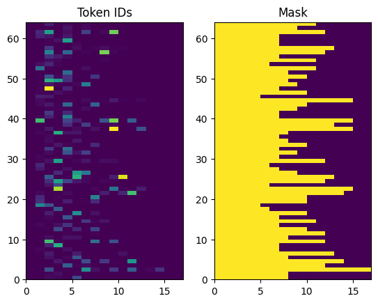
Los ID de token devueltos se rellenan con ceros. Esto se puede convertir fácilmente en una máscara:
plt.subplot(1, 2, 1)
plt.pcolormesh(example_tokens)
plt.title('Token IDs')

plt.subplot(1, 2, 2)
plt.pcolormesh(example_tokens != 0)
plt.title('Mask')
Text(0.5, 1.0, 'Mask')
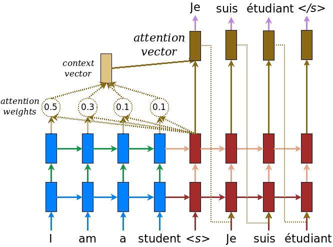
El modelo de codificador / decodificador
El siguiente diagrama muestra una descripción general del modelo. En cada paso de tiempo, la salida del decodificador se combina con una suma ponderada sobre la entrada codificada, para predecir la siguiente palabra. El diagrama y fórmulas son de papel de Luong .
Antes de entrar en él, defina algunas constantes para el modelo:
embedding_dim = 256
units = 1024
El codificador
Empiece por construir el codificador, la parte azul del diagrama de arriba.
El codificador:
- Toma una lista de ID de testigo (de
input_text_processor). - Mira hacia arriba un vector de inclusión para cada ficha (El uso de un
layers.Embedding). - Procesa las incrustaciones en una nueva secuencia (utilizando un
layers.GRU). - Devoluciones:
- La secuencia procesada. Esto se pasará al jefe de atención.
- El estado interno. Esto se utilizará para inicializar el decodificador.
class Encoder(tf.keras.layers.Layer):
  def __init__(self, input_vocab_size, embedding_dim, enc_units):
    super(Encoder, self).__init__()
    self.enc_units = enc_units
    self.input_vocab_size = input_vocab_size

    # The embedding layer converts tokens to vectors
    self.embedding = tf.keras.layers.Embedding(self.input_vocab_size,
                                               embedding_dim)

    # The GRU RNN layer processes those vectors sequentially.
    self.gru = tf.keras.layers.GRU(self.enc_units,
                                   # Return the sequence and state
                                   return_sequences=True,
                                   return_state=True,
                                   recurrent_initializer='glorot_uniform')

  def call(self, tokens, state=None):
    shape_checker = ShapeChecker()
    shape_checker(tokens, ('batch', 's'))

    # 2. The embedding layer looks up the embedding for each token.
    vectors = self.embedding(tokens)
    shape_checker(vectors, ('batch', 's', 'embed_dim'))

    # 3. The GRU processes the embedding sequence.
    #    output shape: (batch, s, enc_units)
    #    state shape: (batch, enc_units)
    output, state = self.gru(vectors, initial_state=state)
    shape_checker(output, ('batch', 's', 'enc_units'))
    shape_checker(state, ('batch', 'enc_units'))

    # 4. Returns the new sequence and its state.
    return output, state
Así es como encaja hasta ahora:
# Convert the input text to tokens.
example_tokens = input_text_processor(example_input_batch)

# Encode the input sequence.
encoder = Encoder(input_text_processor.vocabulary_size(),
                  embedding_dim, units)
example_enc_output, example_enc_state = encoder(example_tokens)

print(f'Input batch, shape (batch): {example_input_batch.shape}')
print(f'Input batch tokens, shape (batch, s): {example_tokens.shape}')
print(f'Encoder output, shape (batch, s, units): {example_enc_output.shape}')
print(f'Encoder state, shape (batch, units): {example_enc_state.shape}')
Input batch, shape (batch): (64,)
Input batch tokens, shape (batch, s): (64, 14)
Encoder output, shape (batch, s, units): (64, 14, 1024)
Encoder state, shape (batch, units): (64, 1024)
El codificador devuelve su estado interno para que su estado se pueda utilizar para inicializar el decodificador.
También es común que un RNN devuelva su estado para que pueda procesar una secuencia en varias llamadas. Verás más de eso construyendo el decodificador.
La cabeza de atención
El decodificador usa la atención para enfocarse selectivamente en partes de la secuencia de entrada. La atención toma una secuencia de vectores como entrada para cada ejemplo y devuelve un vector de "atención" para cada ejemplo. Esta capa atención es similar a un layers.GlobalAveragePoling1D pero la capa atención realiza un promedio ponderado.
Veamos cómo funciona esto:


Donde:
- \(s\) es el índice del codificador.
- \(t\) es el índice de decodificador.
- \(\alpha_{ts}\) es el peso de la atención.
- \(h_s\) es la secuencia de salidas del codificador siendo atendido (la "llave" atención y "valor" en la terminología del transformador).
- \(h_t\) es el estado del decodificador asistir a la secuencia (la "consulta" en la terminología de la atención transformador).
- \(c_t\) es el vector de contexto resultante.
- \(a_t\) es la salida final combinando el "contexto" y "consulta".
Las ecuaciones:
- Calcula los pesos de atención, \(\alpha_{ts}\), como softmax través secuencia de salida del codificador.
- Calcula el vector de contexto como la suma ponderada de las salidas del codificador.
Última es la \(score\) función. Su trabajo es calcular un logit-score escalar para cada par clave-consulta. Hay dos enfoques comunes:
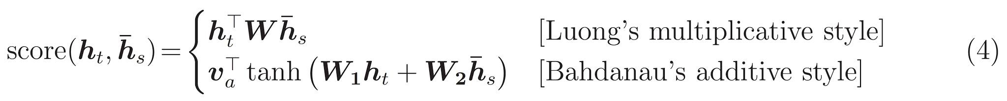
Este tutorial usa la atención aditivo de Bahdanau . TensorFlow incluye implementaciones de tanto como layers.Attention y layers.AdditiveAttention . La clase por debajo de las manijas de las matrices de peso en un par de layers.Dense capas, y llama a la implementación incorporada.
class BahdanauAttention(tf.keras.layers.Layer):
  def __init__(self, units):
    super().__init__()
    # For Eqn. (4), the  Bahdanau attention
    self.W1 = tf.keras.layers.Dense(units, use_bias=False)
    self.W2 = tf.keras.layers.Dense(units, use_bias=False)

    self.attention = tf.keras.layers.AdditiveAttention()

  def call(self, query, value, mask):
    shape_checker = ShapeChecker()
    shape_checker(query, ('batch', 't', 'query_units'))
    shape_checker(value, ('batch', 's', 'value_units'))
    shape_checker(mask, ('batch', 's'))

    # From Eqn. (4), `W1@ht`.
    w1_query = self.W1(query)
    shape_checker(w1_query, ('batch', 't', 'attn_units'))

    # From Eqn. (4), `W2@hs`.
    w2_key = self.W2(value)
    shape_checker(w2_key, ('batch', 's', 'attn_units'))

    query_mask = tf.ones(tf.shape(query)[:-1], dtype=bool)
    value_mask = mask

    context_vector, attention_weights = self.attention(
        inputs = [w1_query, value, w2_key],
        mask=[query_mask, value_mask],
        return_attention_scores = True,
    )
    shape_checker(context_vector, ('batch', 't', 'value_units'))
    shape_checker(attention_weights, ('batch', 't', 's'))

    return context_vector, attention_weights
Prueba la capa de atención
Crear un BahdanauAttention capa:
attention_layer = BahdanauAttention(units)
Esta capa toma 3 entradas:
- La
query: Este será generada por el decodificador, más adelante. - El
value: Esta será la salida del codificador. - La
mask: para excluir el relleno,example_tokens != 0
(example_tokens != 0).shape
TensorShape([64, 14])
La implementación vectorizada de la capa de atención le permite pasar un lote de secuencias de vectores de consulta y un lote de secuencia de vectores de valor. El resultado es:
- Un lote de secuencias de vectores de resultado del tamaño de las consultas.
- A la atención de lote mapas, con tamaño
(query_length, value_length).
# Later, the decoder will generate this attention query
example_attention_query = tf.random.normal(shape=[len(example_tokens), 2, 10])

# Attend to the encoded tokens

context_vector, attention_weights = attention_layer(
    query=example_attention_query,
    value=example_enc_output,
    mask=(example_tokens != 0))

print(f'Attention result shape: (batch_size, query_seq_length, units):           {context_vector.shape}')
print(f'Attention weights shape: (batch_size, query_seq_length, value_seq_length): {attention_weights.shape}')
Attention result shape: (batch_size, query_seq_length, units):           (64, 2, 1024)
Attention weights shape: (batch_size, query_seq_length, value_seq_length): (64, 2, 14)
Los pesos de atención deben sumar a 1.0 para cada secuencia.
Aquí son los pesos de atención a través de las secuencias en t=0 :
plt.subplot(1, 2, 1)
plt.pcolormesh(attention_weights[:, 0, :])
plt.title('Attention weights')

plt.subplot(1, 2, 2)
plt.pcolormesh(example_tokens != 0)
plt.title('Mask')
Text(0.5, 1.0, 'Mask')

Debido a la inicialización de pequeña azar los pesos de atención son todos cerca de 1/(sequence_length) . Si se acerca a los pesos para una sola secuencia, se puede ver que hay una pequeña variación que el modelo puede aprender a ampliar y explotar.
attention_weights.shape
TensorShape([64, 2, 14])
attention_slice = attention_weights[0, 0].numpy()
attention_slice = attention_slice[attention_slice != 0]
plt.suptitle('Attention weights for one sequence')

plt.figure(figsize=(12, 6))
a1 = plt.subplot(1, 2, 1)
plt.bar(range(len(attention_slice)), attention_slice)
# freeze the xlim
plt.xlim(plt.xlim())
plt.xlabel('Attention weights')

a2 = plt.subplot(1, 2, 2)
plt.bar(range(len(attention_slice)), attention_slice)
plt.xlabel('Attention weights, zoomed')

# zoom in
top = max(a1.get_ylim())
zoom = 0.85*top
a2.set_ylim([0.90*top, top])
a1.plot(a1.get_xlim(), [zoom, zoom], color='k')
[<matplotlib.lines.Line2D at 0x7fb42c5b1090>]
<Figure size 432x288 with 0 Axes>

El decodificador
El trabajo del decodificador es generar predicciones para el siguiente token de salida.
- El decodificador recibe la salida completa del codificador.
- Utiliza un RNN para realizar un seguimiento de lo que ha generado hasta ahora.
- Utiliza su salida RNN como la consulta a la atención sobre la salida del codificador, produciendo el vector de contexto.
- Combina la salida RNN y el vector de contexto usando la Ecuación 3 (abajo) para generar el "vector de atención".
- Genera predicciones logit para el siguiente token basado en el "vector de atención".

Aquí está el Decoder clase y su inicializador. El inicializador crea todas las capas necesarias.
class Decoder(tf.keras.layers.Layer):
  def __init__(self, output_vocab_size, embedding_dim, dec_units):
    super(Decoder, self).__init__()
    self.dec_units = dec_units
    self.output_vocab_size = output_vocab_size
    self.embedding_dim = embedding_dim

    # For Step 1. The embedding layer convets token IDs to vectors
    self.embedding = tf.keras.layers.Embedding(self.output_vocab_size,
                                               embedding_dim)

    # For Step 2. The RNN keeps track of what's been generated so far.
    self.gru = tf.keras.layers.GRU(self.dec_units,
                                   return_sequences=True,
                                   return_state=True,
                                   recurrent_initializer='glorot_uniform')

    # For step 3. The RNN output will be the query for the attention layer.
    self.attention = BahdanauAttention(self.dec_units)

    # For step 4. Eqn. (3): converting `ct` to `at`
    self.Wc = tf.keras.layers.Dense(dec_units, activation=tf.math.tanh,
                                    use_bias=False)

    # For step 5. This fully connected layer produces the logits for each
    # output token.
    self.fc = tf.keras.layers.Dense(self.output_vocab_size)
La call método para esta capa toma y devuelve varios tensores. Organícelos en clases de contenedores simples:
class DecoderInput(typing.NamedTuple):
  new_tokens: Any
  enc_output: Any
  mask: Any

class DecoderOutput(typing.NamedTuple):
  logits: Any
  attention_weights: Any
Aquí está la aplicación de la call método:
def call(self,
         inputs: DecoderInput,
         state=None) -> Tuple[DecoderOutput, tf.Tensor]:
  shape_checker = ShapeChecker()
  shape_checker(inputs.new_tokens, ('batch', 't'))
  shape_checker(inputs.enc_output, ('batch', 's', 'enc_units'))
  shape_checker(inputs.mask, ('batch', 's'))

  if state is not None:
    shape_checker(state, ('batch', 'dec_units'))

  # Step 1. Lookup the embeddings
  vectors = self.embedding(inputs.new_tokens)
  shape_checker(vectors, ('batch', 't', 'embedding_dim'))

  # Step 2. Process one step with the RNN
  rnn_output, state = self.gru(vectors, initial_state=state)

  shape_checker(rnn_output, ('batch', 't', 'dec_units'))
  shape_checker(state, ('batch', 'dec_units'))

  # Step 3. Use the RNN output as the query for the attention over the
  # encoder output.
  context_vector, attention_weights = self.attention(
      query=rnn_output, value=inputs.enc_output, mask=inputs.mask)
  shape_checker(context_vector, ('batch', 't', 'dec_units'))
  shape_checker(attention_weights, ('batch', 't', 's'))

  # Step 4. Eqn. (3): Join the context_vector and rnn_output
  #     [ct; ht] shape: (batch t, value_units + query_units)
  context_and_rnn_output = tf.concat([context_vector, rnn_output], axis=-1)

  # Step 4. Eqn. (3): `at = tanh(Wc@[ct; ht])`
  attention_vector = self.Wc(context_and_rnn_output)
  shape_checker(attention_vector, ('batch', 't', 'dec_units'))

  # Step 5. Generate logit predictions:
  logits = self.fc(attention_vector)
  shape_checker(logits, ('batch', 't', 'output_vocab_size'))

  return DecoderOutput(logits, attention_weights), state
Decoder.call = call
El codificador procesa su secuencia de entrada completa con una sola llamada a su RNN. Esta implementación del decodificador puede hacer eso también a un entrenamiento eficiente. Pero este tutorial ejecutará el decodificador en un bucle por algunas razones:
- Flexibilidad: escribir el bucle le da control directo sobre el procedimiento de entrenamiento.
- Claridad: Es posible hacer trucos de enmascaramiento y utilizar
layers.RNNotfa.seq2seqAPI para empacar todo esto en una sola llamada. Pero escribirlo como un bucle puede ser más claro.- Bucle de capacitación gratuita se demuestra en la generación de texto tutiorial.
Ahora intente usar este decodificador.
decoder = Decoder(output_text_processor.vocabulary_size(),
                  embedding_dim, units)
El decodificador toma 4 entradas.
-
new_tokens- La última ficha genera. Inicializar el decodificador con el"[START]"token. -
enc_output- Generado por elEncoder. -
mask- Un tensor de booleano que indica dóndetokens != 0 -
state- El anteriorstatede salida del decodificador (el estado interno de RNN del descodificador). PaseNonede cero inicializarlo. El papel original lo inicializa desde el estado RNN final del codificador.
# Convert the target sequence, and collect the "[START]" tokens
example_output_tokens = output_text_processor(example_target_batch)

start_index = output_text_processor.get_vocabulary().index('[START]')
first_token = tf.constant([[start_index]] * example_output_tokens.shape[0])
# Run the decoder
dec_result, dec_state = decoder(
    inputs = DecoderInput(new_tokens=first_token,
                          enc_output=example_enc_output,
                          mask=(example_tokens != 0)),
    state = example_enc_state
)

print(f'logits shape: (batch_size, t, output_vocab_size) {dec_result.logits.shape}')
print(f'state shape: (batch_size, dec_units) {dec_state.shape}')
logits shape: (batch_size, t, output_vocab_size) (64, 1, 5000)
state shape: (batch_size, dec_units) (64, 1024)
Muestra un token de acuerdo con los logits:
sampled_token = tf.random.categorical(dec_result.logits[:, 0, :], num_samples=1)
Decodifica el token como la primera palabra de la salida:
vocab = np.array(output_text_processor.get_vocabulary())
first_word = vocab[sampled_token.numpy()]
first_word[:5]
array([['already'],
       ['plants'],
       ['pretended'],
       ['convince'],
       ['square']], dtype='<U16')
Ahora use el decodificador para generar un segundo conjunto de logits.
- Pase al mismo
enc_outputymask, éstos no han cambiado. - Pasar el muestreado token como
new_tokens. - Pasar el
decoder_stateel decodificador regresó por última vez, por lo que el RNN continúa con un recuerdo de donde lo dejó la última vez.
dec_result, dec_state = decoder(
    DecoderInput(sampled_token,
                 example_enc_output,
                 mask=(example_tokens != 0)),
    state=dec_state)
sampled_token = tf.random.categorical(dec_result.logits[:, 0, :], num_samples=1)
first_word = vocab[sampled_token.numpy()]
first_word[:5]
array([['nap'],
       ['mean'],
       ['worker'],
       ['passage'],
       ['baked']], dtype='<U16')
Capacitación
Ahora que tiene todos los componentes del modelo, es hora de comenzar a entrenar el modelo. Necesitarás:
- Una función de pérdida y un optimizador para realizar la optimización.
- Una función de paso de entrenamiento que define cómo actualizar el modelo para cada lote de entrada / destino.
- Un circuito de entrenamiento para impulsar el entrenamiento y guardar puntos de control.
Definir la función de pérdida
class MaskedLoss(tf.keras.losses.Loss):
  def __init__(self):
    self.name = 'masked_loss'
    self.loss = tf.keras.losses.SparseCategoricalCrossentropy(
        from_logits=True, reduction='none')

  def __call__(self, y_true, y_pred):
    shape_checker = ShapeChecker()
    shape_checker(y_true, ('batch', 't'))
    shape_checker(y_pred, ('batch', 't', 'logits'))

    # Calculate the loss for each item in the batch.
    loss = self.loss(y_true, y_pred)
    shape_checker(loss, ('batch', 't'))

    # Mask off the losses on padding.
    mask = tf.cast(y_true != 0, tf.float32)
    shape_checker(mask, ('batch', 't'))
    loss *= mask

    # Return the total.
    return tf.reduce_sum(loss)
Implementar el paso de formación
Comienza con una clase del modelo, el proceso de formación se llevará a cabo como el train_step método en este modelo. Véase Personalización de ajuste para más detalles.
Aquí el train_step método es una envoltura alrededor de la _train_step aplicación que vendrá después. Este envoltorio incluye un interruptor para encender y apagar tf.function compilación, para hacer más fácil la depuración.
class TrainTranslator(tf.keras.Model):
  def __init__(self, embedding_dim, units,
               input_text_processor,
               output_text_processor,
               use_tf_function=True):
    super().__init__()
    # Build the encoder and decoder
    encoder = Encoder(input_text_processor.vocabulary_size(),
                      embedding_dim, units)
    decoder = Decoder(output_text_processor.vocabulary_size(),
                      embedding_dim, units)

    self.encoder = encoder
    self.decoder = decoder
    self.input_text_processor = input_text_processor
    self.output_text_processor = output_text_processor
    self.use_tf_function = use_tf_function
    self.shape_checker = ShapeChecker()

  def train_step(self, inputs):
    self.shape_checker = ShapeChecker()
    if self.use_tf_function:
      return self._tf_train_step(inputs)
    else:
      return self._train_step(inputs)
En general, la aplicación de la Model.train_step método es el siguiente:
- Recibir un lote de
input_text, target_textdeltf.data.Dataset. - Convierta esas entradas de texto sin procesar en incrustaciones de tokens y máscaras.
- Ejecutar el codificador en los
input_tokenspara obtener elencoder_outputyencoder_state. - Inicialice el estado y la pérdida del decodificador.
- Lazo sobre los
target_tokens:- Ejecute el decodificador paso a paso.
- Calcula la pérdida de cada paso.
- Acumule la pérdida media.
- Calcular el gradiente de la pérdida y utilizar el optimizador para aplicar cambios a la modelo
trainable_variables.
El _preprocess método, añadido a continuación, ejecuta los pasos # 1 y # 2:
def _preprocess(self, input_text, target_text):
  self.shape_checker(input_text, ('batch',))
  self.shape_checker(target_text, ('batch',))

  # Convert the text to token IDs
  input_tokens = self.input_text_processor(input_text)
  target_tokens = self.output_text_processor(target_text)
  self.shape_checker(input_tokens, ('batch', 's'))
  self.shape_checker(target_tokens, ('batch', 't'))

  # Convert IDs to masks.
  input_mask = input_tokens != 0
  self.shape_checker(input_mask, ('batch', 's'))

  target_mask = target_tokens != 0
  self.shape_checker(target_mask, ('batch', 't'))

  return input_tokens, input_mask, target_tokens, target_mask
TrainTranslator._preprocess = _preprocess
El _train_step método, añadido a continuación, se ocupa de los pasos restantes, excepto para ejecutar realmente el decodificador:
def _train_step(self, inputs):
  input_text, target_text = inputs

  (input_tokens, input_mask,
   target_tokens, target_mask) = self._preprocess(input_text, target_text)

  max_target_length = tf.shape(target_tokens)[1]

  with tf.GradientTape() as tape:
    # Encode the input
    enc_output, enc_state = self.encoder(input_tokens)
    self.shape_checker(enc_output, ('batch', 's', 'enc_units'))
    self.shape_checker(enc_state, ('batch', 'enc_units'))

    # Initialize the decoder's state to the encoder's final state.
    # This only works if the encoder and decoder have the same number of
    # units.
    dec_state = enc_state
    loss = tf.constant(0.0)

    for t in tf.range(max_target_length-1):
      # Pass in two tokens from the target sequence:
      # 1. The current input to the decoder.
      # 2. The target for the decoder's next prediction.
      new_tokens = target_tokens[:, t:t+2]
      step_loss, dec_state = self._loop_step(new_tokens, input_mask,
                                             enc_output, dec_state)
      loss = loss + step_loss

    # Average the loss over all non padding tokens.
    average_loss = loss / tf.reduce_sum(tf.cast(target_mask, tf.float32))

  # Apply an optimization step
  variables = self.trainable_variables
  gradients = tape.gradient(average_loss, variables)
  self.optimizer.apply_gradients(zip(gradients, variables))

  # Return a dict mapping metric names to current value
  return {'batch_loss': average_loss}
TrainTranslator._train_step = _train_step
El _loop_step método, añadido a continuación, ejecuta el decodificador y calcula la pérdida gradual y nuevo estado del decodificador ( dec_state ).
def _loop_step(self, new_tokens, input_mask, enc_output, dec_state):
  input_token, target_token = new_tokens[:, 0:1], new_tokens[:, 1:2]

  # Run the decoder one step.
  decoder_input = DecoderInput(new_tokens=input_token,
                               enc_output=enc_output,
                               mask=input_mask)

  dec_result, dec_state = self.decoder(decoder_input, state=dec_state)
  self.shape_checker(dec_result.logits, ('batch', 't1', 'logits'))
  self.shape_checker(dec_result.attention_weights, ('batch', 't1', 's'))
  self.shape_checker(dec_state, ('batch', 'dec_units'))

  # `self.loss` returns the total for non-padded tokens
  y = target_token
  y_pred = dec_result.logits
  step_loss = self.loss(y, y_pred)

  return step_loss, dec_state
TrainTranslator._loop_step = _loop_step
Prueba el paso de entrenamiento
Construir un TrainTranslator , y configurarlo para entrenar con el Model.compile método:
translator = TrainTranslator(
    embedding_dim, units,
    input_text_processor=input_text_processor,
    output_text_processor=output_text_processor,
    use_tf_function=False)

# Configure the loss and optimizer
translator.compile(
    optimizer=tf.optimizers.Adam(),
    loss=MaskedLoss(),
)
Probar el train_step . Para un modelo de texto como este, la pérdida debería comenzar cerca de:
np.log(output_text_processor.vocabulary_size())
8.517193191416236
%%time
for n in range(10):
  print(translator.train_step([example_input_batch, example_target_batch]))
print()
{'batch_loss': <tf.Tensor: shape=(), dtype=float32, numpy=7.5849695>}
{'batch_loss': <tf.Tensor: shape=(), dtype=float32, numpy=7.55271>}
{'batch_loss': <tf.Tensor: shape=(), dtype=float32, numpy=7.4929113>}
{'batch_loss': <tf.Tensor: shape=(), dtype=float32, numpy=7.3296022>}
{'batch_loss': <tf.Tensor: shape=(), dtype=float32, numpy=6.80437>}
{'batch_loss': <tf.Tensor: shape=(), dtype=float32, numpy=5.000246>}
{'batch_loss': <tf.Tensor: shape=(), dtype=float32, numpy=5.8740363>}
{'batch_loss': <tf.Tensor: shape=(), dtype=float32, numpy=4.794589>}
{'batch_loss': <tf.Tensor: shape=(), dtype=float32, numpy=4.3175836>}
{'batch_loss': <tf.Tensor: shape=(), dtype=float32, numpy=4.108163>}

CPU times: user 5.49 s, sys: 0 ns, total: 5.49 s
Wall time: 5.45 s
Si bien es más fácil de depurar sin tf.function sí da un aumento de rendimiento. Así que ahora que el _train_step método funciona, pruebe el tf.function -wrapped _tf_train_step , para maximizar el rendimiento durante el entrenamiento:
@tf.function(input_signature=[[tf.TensorSpec(dtype=tf.string, shape=[None]),
                               tf.TensorSpec(dtype=tf.string, shape=[None])]])
def _tf_train_step(self, inputs):
  return self._train_step(inputs)
TrainTranslator._tf_train_step = _tf_train_step
translator.use_tf_function = True
La primera llamada será lenta porque rastrea la función.
translator.train_step([example_input_batch, example_target_batch])
2021-12-04 12:09:48.074769: E tensorflow/core/grappler/optimizers/meta_optimizer.cc:812] function_optimizer failed: INVALID_ARGUMENT: Input 6 of node gradient_tape/while/while_grad/body/_531/gradient_tape/while/gradients/while/decoder_1/gru_3/PartitionedCall_grad/PartitionedCall was passed variant from gradient_tape/while/while_grad/body/_531/gradient_tape/while/gradients/while/decoder_1/gru_3/PartitionedCall_grad/TensorListPopBack_2:1 incompatible with expected float.
2021-12-04 12:09:48.180156: E tensorflow/core/grappler/optimizers/meta_optimizer.cc:812] layout failed: OUT_OF_RANGE: src_output = 25, but num_outputs is only 25
2021-12-04 12:09:48.285846: E tensorflow/core/grappler/optimizers/meta_optimizer.cc:812] tfg_optimizer{} failed: INVALID_ARGUMENT: Input 6 of node gradient_tape/while/while_grad/body/_531/gradient_tape/while/gradients/while/decoder_1/gru_3/PartitionedCall_grad/PartitionedCall was passed variant from gradient_tape/while/while_grad/body/_531/gradient_tape/while/gradients/while/decoder_1/gru_3/PartitionedCall_grad/TensorListPopBack_2:1 incompatible with expected float.
    when importing GraphDef to MLIR module in GrapplerHook
2021-12-04 12:09:48.307794: E tensorflow/core/grappler/optimizers/meta_optimizer.cc:812] function_optimizer failed: INVALID_ARGUMENT: Input 6 of node gradient_tape/while/while_grad/body/_531/gradient_tape/while/gradients/while/decoder_1/gru_3/PartitionedCall_grad/PartitionedCall was passed variant from gradient_tape/while/while_grad/body/_531/gradient_tape/while/gradients/while/decoder_1/gru_3/PartitionedCall_grad/TensorListPopBack_2:1 incompatible with expected float.
2021-12-04 12:09:48.425447: W tensorflow/core/common_runtime/process_function_library_runtime.cc:866] Ignoring multi-device function optimization failure: INVALID_ARGUMENT: Input 1 of node while/body/_1/while/TensorListPushBack_56 was passed float from while/body/_1/while/decoder_1/gru_3/PartitionedCall:6 incompatible with expected variant.
{'batch_loss': <tf.Tensor: shape=(), dtype=float32, numpy=4.045638>}
Pero después de que por lo general es 2-3 veces más rápido que el ansioso train_step método:
%%time
for n in range(10):
  print(translator.train_step([example_input_batch, example_target_batch]))
print()
{'batch_loss': <tf.Tensor: shape=(), dtype=float32, numpy=4.1098256>}
{'batch_loss': <tf.Tensor: shape=(), dtype=float32, numpy=4.169871>}
{'batch_loss': <tf.Tensor: shape=(), dtype=float32, numpy=4.139249>}
{'batch_loss': <tf.Tensor: shape=(), dtype=float32, numpy=4.0410743>}
{'batch_loss': <tf.Tensor: shape=(), dtype=float32, numpy=3.9664454>}
{'batch_loss': <tf.Tensor: shape=(), dtype=float32, numpy=3.895707>}
{'batch_loss': <tf.Tensor: shape=(), dtype=float32, numpy=3.8154407>}
{'batch_loss': <tf.Tensor: shape=(), dtype=float32, numpy=3.7583396>}
{'batch_loss': <tf.Tensor: shape=(), dtype=float32, numpy=3.6986444>}
{'batch_loss': <tf.Tensor: shape=(), dtype=float32, numpy=3.640298>}

CPU times: user 4.4 s, sys: 960 ms, total: 5.36 s
Wall time: 1.67 s
Una buena prueba de un nuevo modelo es ver que puede adaptarse a un solo lote de entrada. Pruébelo, la pérdida debería ir rápidamente a cero:
losses = []
for n in range(100):
  print('.', end='')
  logs = translator.train_step([example_input_batch, example_target_batch])
  losses.append(logs['batch_loss'].numpy())

print()
plt.plot(losses)
....................................................................................................
[<matplotlib.lines.Line2D at 0x7fb427edf210>]

Ahora que está seguro de que el paso de entrenamiento está funcionando, cree una copia nueva del modelo para entrenar desde cero:
train_translator = TrainTranslator(
    embedding_dim, units,
    input_text_processor=input_text_processor,
    output_text_processor=output_text_processor)

# Configure the loss and optimizer
train_translator.compile(
    optimizer=tf.optimizers.Adam(),
    loss=MaskedLoss(),
)
Entrena el modelo
Si bien no hay nada malo con la escritura de su propio bucle de formación personalizada, la aplicación de la Model.train_step método, al igual que en el apartado anterior, le permite ejecutar Model.fit y no tener que escribir todo ese código caldera de la placa.
Este tutorial sólo los trenes durante un par de épocas, a fin de utilizar un callbacks.Callback para recoger la historia de las pérdidas por lotes, para el trazado:
class BatchLogs(tf.keras.callbacks.Callback):
  def __init__(self, key):
    self.key = key
    self.logs = []

  def on_train_batch_end(self, n, logs):
    self.logs.append(logs[self.key])

batch_loss = BatchLogs('batch_loss')
train_translator.fit(dataset, epochs=3,
                     callbacks=[batch_loss])
Epoch 1/3
2021-12-04 12:10:11.617839: E tensorflow/core/grappler/optimizers/meta_optimizer.cc:812] function_optimizer failed: INVALID_ARGUMENT: Input 6 of node StatefulPartitionedCall/gradient_tape/while/while_grad/body/_589/gradient_tape/while/gradients/while/decoder_2/gru_5/PartitionedCall_grad/PartitionedCall was passed variant from StatefulPartitionedCall/gradient_tape/while/while_grad/body/_589/gradient_tape/while/gradients/while/decoder_2/gru_5/PartitionedCall_grad/TensorListPopBack_2:1 incompatible with expected float.
2021-12-04 12:10:11.737105: E tensorflow/core/grappler/optimizers/meta_optimizer.cc:812] layout failed: OUT_OF_RANGE: src_output = 25, but num_outputs is only 25
2021-12-04 12:10:11.855054: E tensorflow/core/grappler/optimizers/meta_optimizer.cc:812] tfg_optimizer{} failed: INVALID_ARGUMENT: Input 6 of node StatefulPartitionedCall/gradient_tape/while/while_grad/body/_589/gradient_tape/while/gradients/while/decoder_2/gru_5/PartitionedCall_grad/PartitionedCall was passed variant from StatefulPartitionedCall/gradient_tape/while/while_grad/body/_589/gradient_tape/while/gradients/while/decoder_2/gru_5/PartitionedCall_grad/TensorListPopBack_2:1 incompatible with expected float.
    when importing GraphDef to MLIR module in GrapplerHook
2021-12-04 12:10:11.878896: E tensorflow/core/grappler/optimizers/meta_optimizer.cc:812] function_optimizer failed: INVALID_ARGUMENT: Input 6 of node StatefulPartitionedCall/gradient_tape/while/while_grad/body/_589/gradient_tape/while/gradients/while/decoder_2/gru_5/PartitionedCall_grad/PartitionedCall was passed variant from StatefulPartitionedCall/gradient_tape/while/while_grad/body/_589/gradient_tape/while/gradients/while/decoder_2/gru_5/PartitionedCall_grad/TensorListPopBack_2:1 incompatible with expected float.
2021-12-04 12:10:12.004755: W tensorflow/core/common_runtime/process_function_library_runtime.cc:866] Ignoring multi-device function optimization failure: INVALID_ARGUMENT: Input 1 of node StatefulPartitionedCall/while/body/_59/while/TensorListPushBack_56 was passed float from StatefulPartitionedCall/while/body/_59/while/decoder_2/gru_5/PartitionedCall:6 incompatible with expected variant.
1859/1859 [==============================] - 349s 185ms/step - batch_loss: 2.0443
Epoch 2/3
1859/1859 [==============================] - 350s 188ms/step - batch_loss: 1.0382
Epoch 3/3
1859/1859 [==============================] - 343s 184ms/step - batch_loss: 0.8085
<keras.callbacks.History at 0x7fb42c3eda10>
plt.plot(batch_loss.logs)
plt.ylim([0, 3])
plt.xlabel('Batch #')
plt.ylabel('CE/token')
Text(0, 0.5, 'CE/token')
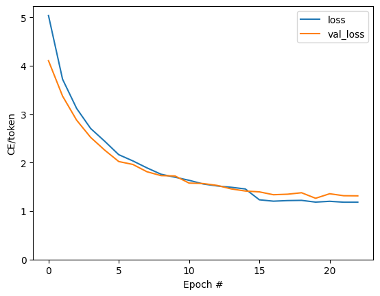
Los saltos visibles en la trama están en los límites de la época.
Traducir
Ahora que el modelo está entrenado, implementar una función para ejecutar la completa text => text de la traducción.
Para este modelo las necesidades para invertir el text => token IDs asignación proporcionada por el output_text_processor . También necesita conocer los ID de los tokens especiales. Todo esto está implementado en el constructor de la nueva clase. Seguirá la implementación del método de traducción real.
En general, esto es similar al ciclo de entrenamiento, excepto que la entrada al decodificador en cada paso de tiempo es una muestra de la última predicción del decodificador.
class Translator(tf.Module):

  def __init__(self, encoder, decoder, input_text_processor,
               output_text_processor):
    self.encoder = encoder
    self.decoder = decoder
    self.input_text_processor = input_text_processor
    self.output_text_processor = output_text_processor

    self.output_token_string_from_index = (
        tf.keras.layers.StringLookup(
            vocabulary=output_text_processor.get_vocabulary(),
            mask_token='',
            invert=True))

    # The output should never generate padding, unknown, or start.
    index_from_string = tf.keras.layers.StringLookup(
        vocabulary=output_text_processor.get_vocabulary(), mask_token='')
    token_mask_ids = index_from_string(['', '[UNK]', '[START]']).numpy()

    token_mask = np.zeros([index_from_string.vocabulary_size()], dtype=np.bool)
    token_mask[np.array(token_mask_ids)] = True
    self.token_mask = token_mask

    self.start_token = index_from_string(tf.constant('[START]'))
    self.end_token = index_from_string(tf.constant('[END]'))
translator = Translator(
    encoder=train_translator.encoder,
    decoder=train_translator.decoder,
    input_text_processor=input_text_processor,
    output_text_processor=output_text_processor,
)
/tmpfs/src/tf_docs_env/lib/python3.7/site-packages/ipykernel_launcher.py:21: DeprecationWarning: `np.bool` is a deprecated alias for the builtin `bool`. To silence this warning, use `bool` by itself. Doing this will not modify any behavior and is safe. If you specifically wanted the numpy scalar type, use `np.bool_` here.
Deprecated in NumPy 1.20; for more details and guidance: https://numpy.org/devdocs/release/1.20.0-notes.html#deprecations
Convertir ID de token en texto
El primer método a aplicar es tokens_to_text que convierte de ID de testigo a texto legible por humanos.
def tokens_to_text(self, result_tokens):
  shape_checker = ShapeChecker()
  shape_checker(result_tokens, ('batch', 't'))
  result_text_tokens = self.output_token_string_from_index(result_tokens)
  shape_checker(result_text_tokens, ('batch', 't'))

  result_text = tf.strings.reduce_join(result_text_tokens,
                                       axis=1, separator=' ')
  shape_checker(result_text, ('batch'))

  result_text = tf.strings.strip(result_text)
  shape_checker(result_text, ('batch',))
  return result_text
Translator.tokens_to_text = tokens_to_text
Ingrese algunos ID de token aleatorios y vea lo que genera:
example_output_tokens = tf.random.uniform(
    shape=[5, 2], minval=0, dtype=tf.int64,
    maxval=output_text_processor.vocabulary_size())
translator.tokens_to_text(example_output_tokens).numpy()
array([b'vain mysteries', b'funny ham', b'drivers responding',
       b'mysterious ignoring', b'fashion votes'], dtype=object)
Muestra de las predicciones del decodificador
Esta función toma las salidas logit del decodificador y muestra los ID de token de esa distribución:
def sample(self, logits, temperature):
  shape_checker = ShapeChecker()
  # 't' is usually 1 here.
  shape_checker(logits, ('batch', 't', 'vocab'))
  shape_checker(self.token_mask, ('vocab',))

  token_mask = self.token_mask[tf.newaxis, tf.newaxis, :]
  shape_checker(token_mask, ('batch', 't', 'vocab'), broadcast=True)

  # Set the logits for all masked tokens to -inf, so they are never chosen.
  logits = tf.where(self.token_mask, -np.inf, logits)

  if temperature == 0.0:
    new_tokens = tf.argmax(logits, axis=-1)
  else:
    logits = tf.squeeze(logits, axis=1)
    new_tokens = tf.random.categorical(logits/temperature,
                                        num_samples=1)

  shape_checker(new_tokens, ('batch', 't'))

  return new_tokens
Translator.sample = sample
Pruebe la ejecución de esta función en algunas entradas aleatorias:
example_logits = tf.random.normal([5, 1, output_text_processor.vocabulary_size()])
example_output_tokens = translator.sample(example_logits, temperature=1.0)
example_output_tokens
<tf.Tensor: shape=(5, 1), dtype=int64, numpy=
array([[4506],
       [3577],
       [2961],
       [4586],
       [ 944]])>
Implementar el ciclo de traducción
Aquí hay una implementación completa del ciclo de traducción de texto a texto.
Esta aplicación recoge los resultados en las listas de Python, antes de usar tf.concat a unirse a ellos en los tensores.
Esta aplicación se desenrolla estáticamente el gráfico a max_length iteraciones. Esto está bien con una ejecución ávida en Python.
def translate_unrolled(self,
                       input_text, *,
                       max_length=50,
                       return_attention=True,
                       temperature=1.0):
  batch_size = tf.shape(input_text)[0]
  input_tokens = self.input_text_processor(input_text)
  enc_output, enc_state = self.encoder(input_tokens)

  dec_state = enc_state
  new_tokens = tf.fill([batch_size, 1], self.start_token)

  result_tokens = []
  attention = []
  done = tf.zeros([batch_size, 1], dtype=tf.bool)

  for _ in range(max_length):
    dec_input = DecoderInput(new_tokens=new_tokens,
                             enc_output=enc_output,
                             mask=(input_tokens!=0))

    dec_result, dec_state = self.decoder(dec_input, state=dec_state)

    attention.append(dec_result.attention_weights)

    new_tokens = self.sample(dec_result.logits, temperature)

    # If a sequence produces an `end_token`, set it `done`
    done = done | (new_tokens == self.end_token)
    # Once a sequence is done it only produces 0-padding.
    new_tokens = tf.where(done, tf.constant(0, dtype=tf.int64), new_tokens)

    # Collect the generated tokens
    result_tokens.append(new_tokens)

    if tf.executing_eagerly() and tf.reduce_all(done):
      break

  # Convert the list of generates token ids to a list of strings.
  result_tokens = tf.concat(result_tokens, axis=-1)
  result_text = self.tokens_to_text(result_tokens)

  if return_attention:
    attention_stack = tf.concat(attention, axis=1)
    return {'text': result_text, 'attention': attention_stack}
  else:
    return {'text': result_text}
Translator.translate = translate_unrolled
Ejecútelo con una entrada simple:
%%time
input_text = tf.constant([
    'hace mucho frio aqui.', # "It's really cold here."
    'Esta es mi vida.', # "This is my life.""
])

result = translator.translate(
    input_text = input_text)

print(result['text'][0].numpy().decode())
print(result['text'][1].numpy().decode())
print()
its a long cold here .
this is my life .

CPU times: user 165 ms, sys: 4.37 ms, total: 169 ms
Wall time: 164 ms
Si desea exportar este modelo que necesita para envolver este método en una tf.function . Esta implementación básica tiene algunos problemas si intenta hacer eso:
- Los gráficos resultantes son muy grandes y tardan unos segundos en crearse, guardar o cargar.
- No se puede romper con un bucle desenrollado de forma estática, por lo que siempre se ejecutará
max_lengthiteraciones, incluso si se realizan todas las salidas. Pero incluso entonces es un poco más rápido que una ejecución ansiosa.
@tf.function(input_signature=[tf.TensorSpec(dtype=tf.string, shape=[None])])
def tf_translate(self, input_text):
  return self.translate(input_text)

Translator.tf_translate = tf_translate
Ejecutar el tf.function vez para compilarlo:
%%time
result = translator.tf_translate(
    input_text = input_text)
CPU times: user 18.8 s, sys: 0 ns, total: 18.8 s
Wall time: 18.7 s
%%time
result = translator.tf_translate(
    input_text = input_text)

print(result['text'][0].numpy().decode())
print(result['text'][1].numpy().decode())
print()
its very cold here .
this is my life .

CPU times: user 175 ms, sys: 0 ns, total: 175 ms
Wall time: 88 ms
[Opcional] Utilice un bucle simbólico
def translate_symbolic(self,
                       input_text,
                       *,
                       max_length=50,
                       return_attention=True,
                       temperature=1.0):
  shape_checker = ShapeChecker()
  shape_checker(input_text, ('batch',))

  batch_size = tf.shape(input_text)[0]

  # Encode the input
  input_tokens = self.input_text_processor(input_text)
  shape_checker(input_tokens, ('batch', 's'))

  enc_output, enc_state = self.encoder(input_tokens)
  shape_checker(enc_output, ('batch', 's', 'enc_units'))
  shape_checker(enc_state, ('batch', 'enc_units'))

  # Initialize the decoder
  dec_state = enc_state
  new_tokens = tf.fill([batch_size, 1], self.start_token)
  shape_checker(new_tokens, ('batch', 't1'))

  # Initialize the accumulators
  result_tokens = tf.TensorArray(tf.int64, size=1, dynamic_size=True)
  attention = tf.TensorArray(tf.float32, size=1, dynamic_size=True)
  done = tf.zeros([batch_size, 1], dtype=tf.bool)
  shape_checker(done, ('batch', 't1'))

  for t in tf.range(max_length):
    dec_input = DecoderInput(
        new_tokens=new_tokens, enc_output=enc_output, mask=(input_tokens != 0))

    dec_result, dec_state = self.decoder(dec_input, state=dec_state)

    shape_checker(dec_result.attention_weights, ('batch', 't1', 's'))
    attention = attention.write(t, dec_result.attention_weights)

    new_tokens = self.sample(dec_result.logits, temperature)
    shape_checker(dec_result.logits, ('batch', 't1', 'vocab'))
    shape_checker(new_tokens, ('batch', 't1'))

    # If a sequence produces an `end_token`, set it `done`
    done = done | (new_tokens == self.end_token)
    # Once a sequence is done it only produces 0-padding.
    new_tokens = tf.where(done, tf.constant(0, dtype=tf.int64), new_tokens)

    # Collect the generated tokens
    result_tokens = result_tokens.write(t, new_tokens)

    if tf.reduce_all(done):
      break

  # Convert the list of generated token ids to a list of strings.
  result_tokens = result_tokens.stack()
  shape_checker(result_tokens, ('t', 'batch', 't0'))
  result_tokens = tf.squeeze(result_tokens, -1)
  result_tokens = tf.transpose(result_tokens, [1, 0])
  shape_checker(result_tokens, ('batch', 't'))

  result_text = self.tokens_to_text(result_tokens)
  shape_checker(result_text, ('batch',))

  if return_attention:
    attention_stack = attention.stack()
    shape_checker(attention_stack, ('t', 'batch', 't1', 's'))

    attention_stack = tf.squeeze(attention_stack, 2)
    shape_checker(attention_stack, ('t', 'batch', 's'))

    attention_stack = tf.transpose(attention_stack, [1, 0, 2])
    shape_checker(attention_stack, ('batch', 't', 's'))

    return {'text': result_text, 'attention': attention_stack}
  else:
    return {'text': result_text}
Translator.translate = translate_symbolic
La implementación inicial usó listas de Python para recopilar los resultados. Esto utiliza tf.range como el iterador de bucle, lo que permite tf.autograph para convertir el bucle. El mayor cambio en esta aplicación es el uso de tf.TensorArray en lugar de pitón list de los tensores se acumulan. tf.TensorArray se requiere para recoger un número variable de tensores en modo gráfico.
Con una ejecución ávida, esta implementación funciona a la par con la original:
%%time
result = translator.translate(
    input_text = input_text)

print(result['text'][0].numpy().decode())
print(result['text'][1].numpy().decode())
print()
its very cold here .
this is my life .

CPU times: user 175 ms, sys: 0 ns, total: 175 ms
Wall time: 170 ms
Pero cuando se envuelve en un tf.function usted notará dos diferencias.
@tf.function(input_signature=[tf.TensorSpec(dtype=tf.string, shape=[None])])
def tf_translate(self, input_text):
  return self.translate(input_text)

Translator.tf_translate = tf_translate
En primer lugar: la creación Graph es mucho más rápido (~ 10 veces), ya que no crea max_iterations copias del modelo.
%%time
result = translator.tf_translate(
    input_text = input_text)
CPU times: user 1.79 s, sys: 0 ns, total: 1.79 s
Wall time: 1.77 s
Segundo: la función compilada es mucho más rápida en entradas pequeñas (5x en este ejemplo), porque puede salirse del bucle.
%%time
result = translator.tf_translate(
    input_text = input_text)

print(result['text'][0].numpy().decode())
print(result['text'][1].numpy().decode())
print()
its very cold here .
this is my life .

CPU times: user 40.1 ms, sys: 0 ns, total: 40.1 ms
Wall time: 17.1 ms
Visualiza el proceso
Los pesos de atención devueltos por el translate demostración del método de donde estaba el modelo de "mirar" cuando se genera cada símbolo de salida.
Entonces, la suma de la atención sobre la entrada debería devolver todos unos:
a = result['attention'][0]

print(np.sum(a, axis=-1))
[1.0000001 0.99999994 1. 0.99999994 1. 0.99999994]
Aquí está la distribución de atención para el primer paso de salida del primer ejemplo. Observe cómo la atención ahora está mucho más enfocada que para el modelo no capacitado:
_ = plt.bar(range(len(a[0, :])), a[0, :])

Dado que existe una alineación aproximada entre las palabras de entrada y salida, espera que la atención se centre cerca de la diagonal:
plt.imshow(np.array(a), vmin=0.0)
<matplotlib.image.AxesImage at 0x7faf2886ced0>

Aquí hay un código para hacer una mejor gráfica de atención:
Parcelas de atención etiquetadas
def plot_attention(attention, sentence, predicted_sentence):
  sentence = tf_lower_and_split_punct(sentence).numpy().decode().split()
  predicted_sentence = predicted_sentence.numpy().decode().split() + ['[END]']
  fig = plt.figure(figsize=(10, 10))
  ax = fig.add_subplot(1, 1, 1)

  attention = attention[:len(predicted_sentence), :len(sentence)]

  ax.matshow(attention, cmap='viridis', vmin=0.0)

  fontdict = {'fontsize': 14}

  ax.set_xticklabels([''] + sentence, fontdict=fontdict, rotation=90)
  ax.set_yticklabels([''] + predicted_sentence, fontdict=fontdict)

  ax.xaxis.set_major_locator(ticker.MultipleLocator(1))
  ax.yaxis.set_major_locator(ticker.MultipleLocator(1))

  ax.set_xlabel('Input text')
  ax.set_ylabel('Output text')
  plt.suptitle('Attention weights')
i=0
plot_attention(result['attention'][i], input_text[i], result['text'][i])
/tmpfs/src/tf_docs_env/lib/python3.7/site-packages/ipykernel_launcher.py:14: UserWarning: FixedFormatter should only be used together with FixedLocator

/tmpfs/src/tf_docs_env/lib/python3.7/site-packages/ipykernel_launcher.py:15: UserWarning: FixedFormatter should only be used together with FixedLocator
  from ipykernel import kernelapp as app
Traduce algunas oraciones más y grábalas:
%%time
three_input_text = tf.constant([
# This is my life.
'Esta es mi vida.',
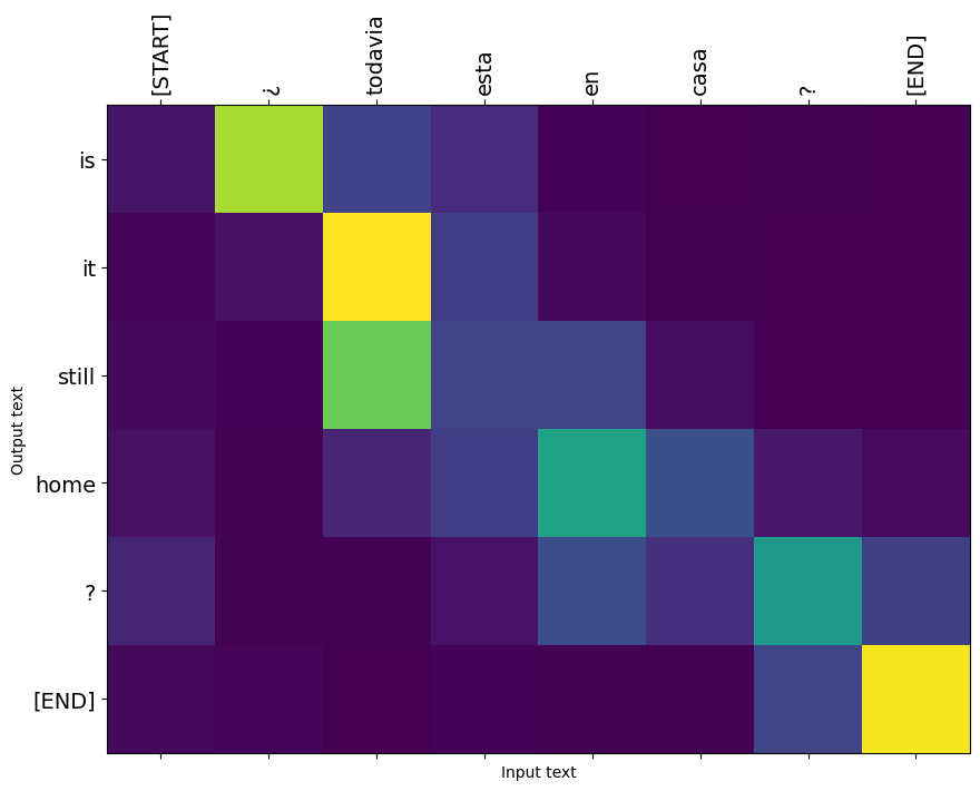
# Are they still home?
'¿Todavía están en casa?',
# Try to find out.'
'Tratar de descubrir.',
])
result = translator.tf_translate(three_input_text)
for tr in result['text']:
print(tr.numpy().decode())
print()
this is my life .
are you still at home ?
all about killed .

CPU times: user 78 ms, sys: 23 ms, total: 101 ms
Wall time: 23.1 ms
result['text']
<tf.Tensor: shape=(3,), dtype=string, numpy=
array([b'this is my life .', b'are you still at home ?',
       b'all about killed .'], dtype=object)>
i = 0
plot_attention(result['attention'][i], three_input_text[i], result['text'][i])
/tmpfs/src/tf_docs_env/lib/python3.7/site-packages/ipykernel_launcher.py:14: UserWarning: FixedFormatter should only be used together with FixedLocator

/tmpfs/src/tf_docs_env/lib/python3.7/site-packages/ipykernel_launcher.py:15: UserWarning: FixedFormatter should only be used together with FixedLocator
  from ipykernel import kernelapp as app

i = 1
plot_attention(result['attention'][i], three_input_text[i], result['text'][i])
/tmpfs/src/tf_docs_env/lib/python3.7/site-packages/ipykernel_launcher.py:14: UserWarning: FixedFormatter should only be used together with FixedLocator

/tmpfs/src/tf_docs_env/lib/python3.7/site-packages/ipykernel_launcher.py:15: UserWarning: FixedFormatter should only be used together with FixedLocator
  from ipykernel import kernelapp as app

i = 2
plot_attention(result['attention'][i], three_input_text[i], result['text'][i])
/tmpfs/src/tf_docs_env/lib/python3.7/site-packages/ipykernel_launcher.py:14: UserWarning: FixedFormatter should only be used together with FixedLocator

/tmpfs/src/tf_docs_env/lib/python3.7/site-packages/ipykernel_launcher.py:15: UserWarning: FixedFormatter should only be used together with FixedLocator
  from ipykernel import kernelapp as app

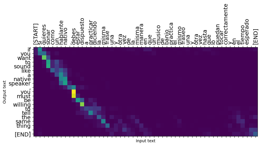
Las oraciones cortas a menudo funcionan bien, pero si la entrada es demasiado larga, el modelo literalmente pierde el enfoque y deja de proporcionar predicciones razonables. Existen dos motivos principales para esto:
- El modelo se entrenó con la alimentación forzada del maestro con la ficha correcta en cada paso, independientemente de las predicciones del modelo. El modelo podría hacerse más robusto si a veces se alimentara de sus propias predicciones.
- El modelo solo tiene acceso a su salida anterior a través del estado RNN. Si el estado de RNN se corrompe, no hay forma de que el modelo se recupere. Transformadores de resolver esto mediante el uso de auto-atención en el codificador y decodificador.
long_input_text = tf.constant([inp[-1]])

import textwrap
print('Expected output:\n', '\n'.join(textwrap.wrap(targ[-1])))
Expected output:
 If you want to sound like a native speaker, you must be willing to
practice saying the same sentence over and over in the same way that
banjo players practice the same phrase over and over until they can
play it correctly and at the desired tempo.
result = translator.tf_translate(long_input_text)

i = 0
plot_attention(result['attention'][i], long_input_text[i], result['text'][i])
_ = plt.suptitle('This never works')
/tmpfs/src/tf_docs_env/lib/python3.7/site-packages/ipykernel_launcher.py:14: UserWarning: FixedFormatter should only be used together with FixedLocator

/tmpfs/src/tf_docs_env/lib/python3.7/site-packages/ipykernel_launcher.py:15: UserWarning: FixedFormatter should only be used together with FixedLocator
  from ipykernel import kernelapp as app
Exportar
Una vez que tenga un modelo que está satisfecho con usted podría querer exportarlo como tf.saved_model para su uso fuera de este programa en Python que lo creó.
Puesto que el modelo es una subclase de tf.Module (a través de keras.Model ), y toda la funcionalidad para la exportación se compila en un tf.function el modelo debe exportar limpiamente con tf.saved_model.save :
Ahora que la función ha sido trazada se puede exportar utilizando saved_model.save :
tf.saved_model.save(translator, 'translator',
                    signatures={'serving_default': translator.tf_translate})
2021-12-04 12:27:54.310890: W tensorflow/python/util/util.cc:368] Sets are not currently considered sequences, but this may change in the future, so consider avoiding using them.
WARNING:absl:Found untraced functions such as encoder_2_layer_call_fn, encoder_2_layer_call_and_return_conditional_losses, decoder_2_layer_call_fn, decoder_2_layer_call_and_return_conditional_losses, embedding_4_layer_call_fn while saving (showing 5 of 60). These functions will not be directly callable after loading.
INFO:tensorflow:Assets written to: translator/assets
INFO:tensorflow:Assets written to: translator/assets
reloaded = tf.saved_model.load('translator')
result = reloaded.tf_translate(three_input_text)
%%time
result = reloaded.tf_translate(three_input_text)

for tr in result['text']:
  print(tr.numpy().decode())

print()
this is my life .
are you still at home ?
find out about to find out .

CPU times: user 42.8 ms, sys: 7.69 ms, total: 50.5 ms
Wall time: 20 ms
Próximos pasos
- Descargar un conjunto de datos diferente a experimentar con traducciones, por ejemplo, Inglés al Alemán, Francés o Inglés a.
- Experimente con el entrenamiento en un conjunto de datos más grande o usando más épocas.
- Probar el transformador tutorial que implementa una tarea de traducción similar, pero utiliza un transformador de capas en lugar de RNNs. Esta versión también utiliza un
text.BertTokenizerpara implementar tokenización wordpiece. - Echar un vistazo a la tensorflow_addons.seq2seq para la implementación de este tipo de secuencia a secuencia modelo. El
tfa.seq2seqpaquete incluye la funcionalidad de nivel superior comoseq2seq.BeamSearchDecoder.