TensorFlow is back at Google I/O on May 14! Register now

Copulas Primer

View on TensorFlow.org

Run in Google Colab

View source on GitHub

Download notebook

import numpy as np
import matplotlib.pyplot as plt
import tensorflow.compat.v2 as tf
tf.enable_v2_behavior()

import tensorflow_probability as tfp
tfd = tfp.distributions
tfb = tfp.bijectors

A [copula](https://en.wikipedia.org/wiki/Copula_(probability_theory%29) is a classical approach for capturing the dependence between random variables. More formally, a copula is a multivariate distribution \(C(U_1, U_2, ...., U_n)\) such that marginalizing gives \(U_i \sim \text{Uniform}(0, 1)\).

Copulas are interesting because we can use them to create multivariate distributions with arbitrary marginals. This is the recipe:

Using the Probability Integral Transform turns an arbitrary continuous R.V. \(X\) into a uniform one \(F_X(X)\), where \(F_X\) is the CDF of \(X\).
Given a copula (say bivariate) \(C(U, V)\), we have that \(U\) and \(V\) have uniform marginal distributions.
Now given our R.V's of interest \(X, Y\), create a new distribution \(C'(X, Y) = C(F_X(X), F_Y(Y))\). The marginals for \(X\) and \(Y\) are the ones we desired.

Marginals are univariate and thus may be easier to measure and/or model. A copula enables starting from marginals yet also achieving arbitrary correlation between dimensions.

Gaussian Copula

To illustrate how copulas are constructed, consider the case of capturing dependence according to multivariate Gaussian correlations. A Gaussian Copula is one given by \(C(u_1, u_2, ...u_n) = \Phi_\Sigma(\Phi^{-1}(u_1), \Phi^{-1}(u_2), ... \Phi^{-1}(u_n))\) where \(\Phi_\Sigma\) represents the CDF of a MultivariateNormal, with covariance \(\Sigma\) and mean 0, and \(\Phi^{-1}\) is the inverse CDF for the standard normal.

Applying the normal's inverse CDF warps the uniform dimensions to be normally distributed. Applying the multivariate normal's CDF then squashes the distribution to be marginally uniform and with Gaussian correlations.

Thus, what we get is that the Gaussian Copula is a distribution over the unit hypercube \([0, 1]^n\) with uniform marginals.

Defined as such, the Gaussian Copula can be implemented with tfd.TransformedDistribution and appropriate Bijector. That is, we are transforming a MultivariateNormal, via the use of the Normal distribution's inverse CDF, implemented by the tfb.NormalCDF bijector.

Below, we implement a Gaussian Copula with one simplifying assumption: that the covariance is parameterized by a Cholesky factor (hence a covariance for MultivariateNormalTriL). (One could use other tf.linalg.LinearOperators to encode different matrix-free assumptions.).

class GaussianCopulaTriL(tfd.TransformedDistribution):
  """Takes a location, and lower triangular matrix for the Cholesky factor."""
  def __init__(self, loc, scale_tril):
    super(GaussianCopulaTriL, self).__init__(
        distribution=tfd.MultivariateNormalTriL(
            loc=loc,
            scale_tril=scale_tril),
        bijector=tfb.NormalCDF(),
        validate_args=False,
        name="GaussianCopulaTriLUniform")


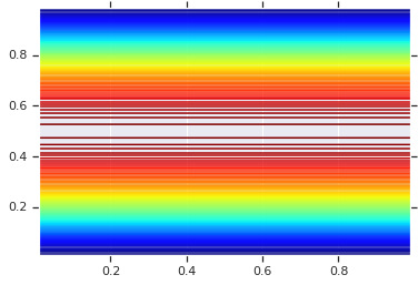
# Plot an example of this.
unit_interval = np.linspace(0.01, 0.99, num=200, dtype=np.float32)
x_grid, y_grid = np.meshgrid(unit_interval, unit_interval)
coordinates = np.concatenate(
    [x_grid[..., np.newaxis],
     y_grid[..., np.newaxis]], axis=-1)

pdf = GaussianCopulaTriL(
    loc=[0., 0.],
    scale_tril=[[1., 0.8], [0., 0.6]],
).prob(coordinates)

# Plot its density.

plt.contour(x_grid, y_grid, pdf, 100, cmap=plt.cm.jet);

png

The power, however, from such a model is using the Probability Integral Transform, to use the copula on arbitrary R.V.s. In this way, we can specify arbitrary marginals, and use the copula to stitch them together.

We start with a model:

\[\begin{align*} X &\sim \text{Kumaraswamy}(a, b) \\ Y &\sim \text{Gumbel}(\mu, \beta) \end{align*}\]

and use the copula to get a bivariate R.V. \(Z\), which has marginals Kumaraswamy and Gumbel.

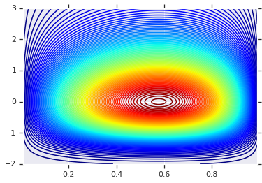
We'll start by plotting the product distribution generated by those two R.V.s. This is just to serve as a comparison point to when we apply the Copula.

a = 2.0
b = 2.0
gloc = 0.
gscale = 1.

x = tfd.Kumaraswamy(a, b)
y = tfd.Gumbel(loc=gloc, scale=gscale)

# Plot the distributions, assuming independence
x_axis_interval = np.linspace(0.01, 0.99, num=200, dtype=np.float32)
y_axis_interval = np.linspace(-2., 3., num=200, dtype=np.float32)
x_grid, y_grid = np.meshgrid(x_axis_interval, y_axis_interval)

pdf = x.prob(x_grid) * y.prob(y_grid)

# Plot its density

plt.contour(x_grid, y_grid, pdf, 100, cmap=plt.cm.jet);

png

Joint Distribution with Different Marginals

Now we use a Gaussian copula to couple the distributions together, and plot that. Again our tool of choice is TransformedDistribution applying the appropriate Bijector to obtain the chosen marginals.

Specifically, we use a Blockwise bijector which applies different bijectors at different parts of the vector (which is still a bijective transformation).

Now we can define the Copula we want. Given a list of target marginals (encoded as bijectors), we can easily construct a new distribution that uses the copula and has the specified marginals.

class WarpedGaussianCopula(tfd.TransformedDistribution):
  """Application of a Gaussian Copula on a list of target marginals.

  This implements an application of a Gaussian Copula. Given [x_0, ... x_n]
  which are distributed marginally (with CDF) [F_0, ... F_n],
  `GaussianCopula` represents an application of the Copula, such that the
  resulting multivariate distribution has the above specified marginals.

  The marginals are specified by `marginal_bijectors`: These are
  bijectors whose `inverse` encodes the CDF and `forward` the inverse CDF.

  block_sizes is a 1-D Tensor to determine splits for `marginal_bijectors`
  length should be same as length of `marginal_bijectors`.
  See tfb.Blockwise for details
  """
  def __init__(self, loc, scale_tril, marginal_bijectors, block_sizes=None):
    super(WarpedGaussianCopula, self).__init__(
        distribution=GaussianCopulaTriL(loc=loc, scale_tril=scale_tril),
        bijector=tfb.Blockwise(bijectors=marginal_bijectors,
                               block_sizes=block_sizes),
        validate_args=False,
        name="GaussianCopula")

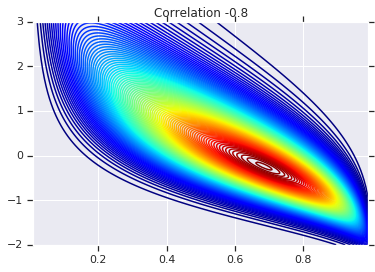
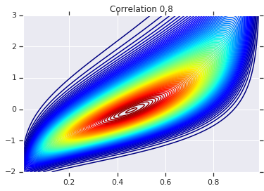
Finally, let's actually use this Gaussian Copula. We'll use a Cholesky of \(\begin{bmatrix}1 & 0\\\rho & \sqrt{(1-\rho^2)}\end{bmatrix}\), which will correspond to variances 1, and correlation \(\rho\) for the multivariate normal.

We'll look at a few cases:

# Create our coordinates:
coordinates = np.concatenate(
    [x_grid[..., np.newaxis], y_grid[..., np.newaxis]], -1)


def create_gaussian_copula(correlation):
  # Use Gaussian Copula to add dependence.
  return WarpedGaussianCopula(
      loc=[0.,  0.],
      scale_tril=[[1., 0.], [correlation, tf.sqrt(1. - correlation ** 2)]],
      # These encode the marginals we want. In this case we want X_0 has
      # Kumaraswamy marginal, and X_1 has Gumbel marginal.

      marginal_bijectors=[
          tfb.Invert(tfb.KumaraswamyCDF(a, b)),
          tfb.Invert(tfb.GumbelCDF(loc=0., scale=1.))])


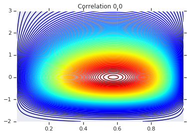
# Note that the zero case will correspond to independent marginals!
correlations = [0., -0.8, 0.8]
copulas = []
probs = []
for correlation in correlations:
  copula = create_gaussian_copula(correlation)
  copulas.append(copula)
  probs.append(copula.prob(coordinates))


# Plot it's density

for correlation, copula_prob in zip(correlations, probs):
  plt.figure()
  plt.contour(x_grid, y_grid, copula_prob, 100, cmap=plt.cm.jet)
  plt.title('Correlation {}'.format(correlation))

png

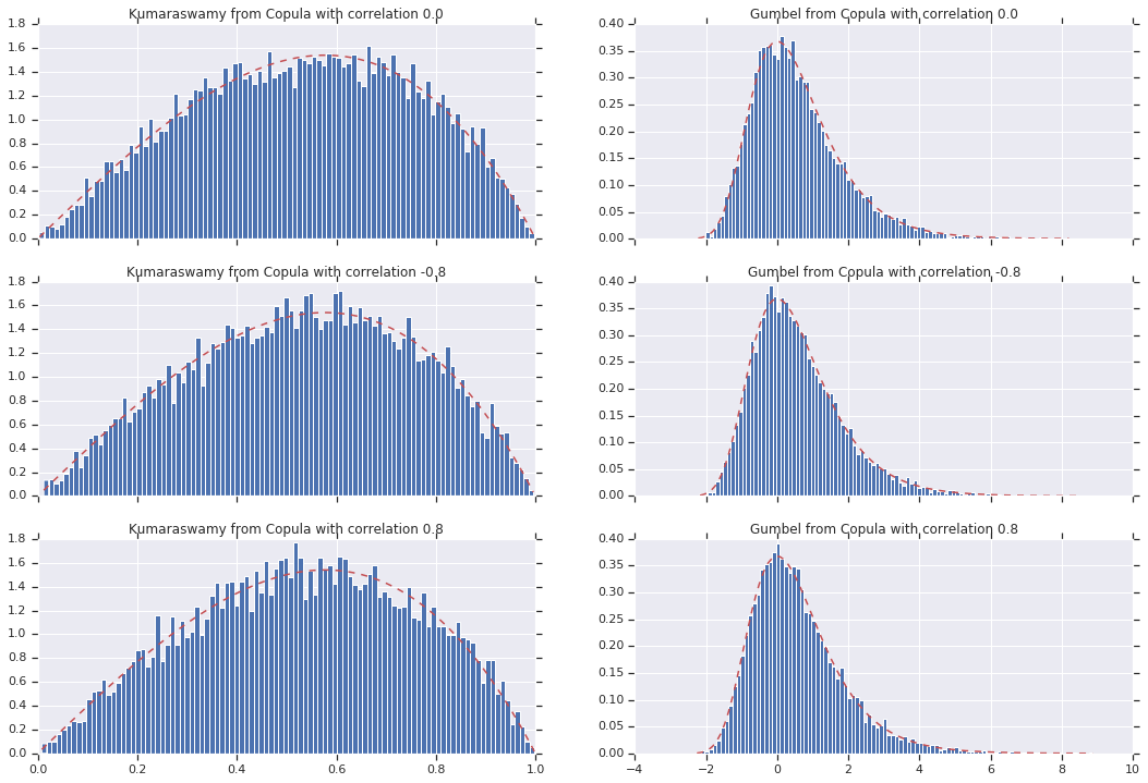
Finally, let's verify that we actually get the marginals we want.

def kumaraswamy_pdf(x):
    return tfd.Kumaraswamy(a, b).prob(np.float32(x))

def gumbel_pdf(x):
    return tfd.Gumbel(gloc, gscale).prob(np.float32(x))


copula_samples = []
for copula in copulas:
  copula_samples.append(copula.sample(10000))

plot_rows = len(correlations)
plot_cols = 2  # for 2  densities [kumarswamy, gumbel]
fig, axes = plt.subplots(plot_rows, plot_cols, sharex='col', figsize=(18,12))

# Let's marginalize out on each, and plot the samples.

for i, (correlation, copula_sample) in enumerate(zip(correlations, copula_samples)):
  k = copula_sample[..., 0].numpy()
  g = copula_sample[..., 1].numpy()


  _, bins, _ = axes[i, 0].hist(k, bins=100, density=True)
  axes[i, 0].plot(bins, kumaraswamy_pdf(bins), 'r--')
  axes[i, 0].set_title('Kumaraswamy from Copula with correlation {}'.format(correlation))

  _, bins, _ = axes[i, 1].hist(g, bins=100, density=True)
  axes[i, 1].plot(bins, gumbel_pdf(bins), 'r--')
  axes[i, 1].set_title('Gumbel from Copula with correlation {}'.format(correlation))

png

Conclusion

And there we go! We've demonstrated that we can construct Gaussian Copulas using the Bijector API.

More generally, writing bijectors using the Bijector API and composing them with a distribution, can create rich families of distributions for flexible modelling.