
|
|
|
 View source on GitHub View source on GitHub
|
|
Latent variable models attempt to capture hidden structure in high dimensional data. Examples include principle component analysis (PCA) and factor analysis. Gaussian processes are "non-parametric" models which can flexibly capture local correlation structure and uncertainty. The Gaussian process latent variable model (Lawrence, 2004) combines these concepts.
Background: Gaussian Processes
A Gaussian process is any collection of random variables such that the marginal distribution over any finite subset is a multivariate normal distribution. For a detailed look at GPs in the context of regression, check out Gaussian Process Regression in TensorFlow Probability.
We use a so-called index set to label each of the random variables in the collection that the GP comprises. In the case of a finite index set, we just get a multivariate normal. GP's are most interesting, though, when we consider infinite collections. In the case of index sets like \(\mathbb{R}^D\), where we have a random variable for every point in \(D\)-dimensional space, the GP can be thought of as a distribution over random functions. A single draw from such a GP, if it could be realized, would assign a (jointly normally-distributed) value to every point in \(\mathbb{R}^D\). In this colab, we'll focus on GP's over some \(\mathbb{R}^D\).
Normal distributions are completely determined by their first and second order statistics -- indeed, one way to define the normal distribution is as one whose higher-order cumulants are all zero. This is the case for GP's, too: we completely specify a GP by describing the mean and covariance*. Recall that for finite-dimensional multivariate normals, the mean is a vector and the covariance is a square, symmetric positive-definite matrix. In the infinite-dimensional GP, these structures generalize to a mean function \(m : \mathbb{R}^D \to \mathbb{R}\), defined at each point of the index set, and a covariance "kernel" function, \(k : \mathbb{R}^D \times \mathbb{R}^D \to \mathbb{R}\). The kernel function is required to be positive-definite, which essentially says that, restricted to a finite set of points, it yields a postiive-definite matrix.
Most of the structure of a GP derives from its covariance kernel function -- this function describes how the values of sampeld functions vary across nearby (or not-so-nearby) points. Different covariance functions encourage different degrees of smoothness. One commonly used kernel function is the "exponentiated quadratic" (a.k.a., "gaussian", "squared exponential" or "radial basis function"), \(k(x, x') = \sigma^2 e^{(x - x^2) / \lambda^2}\). Other examples are outlined on David Duvenaud's kernel cookbook page, as well as in the canonical text Gaussian Processes for Machine Learning.
* With an infinite index set, we also require a consistency condition. Since the definition of the GP is in terms of finite marginals, we must require that these marginals are consistent irrespective of the order in which the marginals are taken. This is a somewhat advanced topic in the theory of stochastic processes, out of scope for this tutorial; suffice it to say things work out ok in the end!
Applying GPs: Regression and Latent Variable Models
One way we can use GPs is for regression: given a bunch of observed data in the form of inputs \(\{x_i\}_{i=1}^N\) (elements of the index set) and observations \(\{y_i\}_{i=1}^N\), we can use these to form a posterior predictive distribution at a new set of points \(\{x_j^*\}_{j=1}^M\). Since the distributions are all Gaussian, this boils down to some straightforward linear algebra (but note: the requisite computations have runtime cubic in the number of data points and require space quadratic in the number of data points -- this is a major limiting factor in the use of GPs and much current research focuses on computationally viable alternatives to exact posterior inference). We cover GP regression in more detail in the GP Regression in TFP colab.
Another way we can use GPs is as a latent variable model: given a collection of high-dimensional observations (e.g., images), we can posit some low-dimensional latent structure. We assume that, conditional on the latent structure, the large number of outputs (pixels in the image) are independent of each other. Training in this model consists of
- optimizing model parameters (kernel function parameters as well as, e.g., observation noise variance), and
- finding, for each training observation (image), a corresponding point location in the index set. All of the optimization can be done by maximizing the marginal log likelihood of the data.
Imports
import numpy as np
import tensorflow as tf
import tf_keras
import tensorflow_probability as tfp
tfd = tfp.distributions
tfk = tfp.math.psd_kernels
%pylab inline
Populating the interactive namespace from numpy and matplotlib
Load MNIST Data
# Load the MNIST data set and isolate a subset of it.
(x_train, y_train), (_, _) = tf_keras.datasets.mnist.load_data()
N = 1000
small_x_train = x_train[:N, ...].astype(np.float64) / 256.
small_y_train = y_train[:N]
Downloading data from https://storage.googleapis.com/tensorflow/tf-keras-datasets/mnist.npz
11493376/11490434 [==============================] - 0s 0us/step
11501568/11490434 [==============================] - 0s 0us/step
Prepare trainable variables
We'll be jointly training 3 model parameters as well as the latent inputs.
# Create some trainable model parameters. We will constrain them to be strictly
# positive when constructing the kernel and the GP.
unconstrained_amplitude = tf.Variable(np.float64(1.), name='amplitude')
unconstrained_length_scale = tf.Variable(np.float64(1.), name='length_scale')
unconstrained_observation_noise = tf.Variable(np.float64(1.), name='observation_noise')
# We need to flatten the images and, somewhat unintuitively, transpose from
# shape [100, 784] to [784, 100]. This is because the 784 pixels will be
# treated as *independent* conditioned on the latent inputs, meaning we really
# have a batch of 784 GP's with 100 index_points.
observations_ = small_x_train.reshape(N, -1).transpose()

# Create a collection of N 2-dimensional index points that will represent our
# latent embeddings of the data. (Lawrence, 2004) prescribes initializing these
# with PCA, but a random initialization actually gives not-too-bad results, so
# we use this for simplicity. For a fun exercise, try doing the
# PCA-initialization yourself!
init_ = np.random.normal(size=(N, 2))
latent_index_points = tf.Variable(init_, name='latent_index_points')
Construct model and training ops
# Create our kernel and GP distribution
EPS = np.finfo(np.float64).eps

def create_kernel():
  amplitude = tf.math.softplus(EPS + unconstrained_amplitude)
  length_scale = tf.math.softplus(EPS + unconstrained_length_scale)
  kernel = tfk.ExponentiatedQuadratic(amplitude, length_scale)
  return kernel

def loss_fn():
  observation_noise_variance = tf.math.softplus(
      EPS + unconstrained_observation_noise)
  gp = tfd.GaussianProcess(
      kernel=create_kernel(),
      index_points=latent_index_points,
      observation_noise_variance=observation_noise_variance)
  log_probs = gp.log_prob(observations_, name='log_prob')
  return -tf.reduce_mean(log_probs)

trainable_variables = [unconstrained_amplitude,
                       unconstrained_length_scale,
                       unconstrained_observation_noise,
                       latent_index_points]

optimizer = tf_keras.optimizers.Adam(learning_rate=1.0)

@tf.function(autograph=False, jit_compile=True)
def train_model():
  with tf.GradientTape() as tape:
    loss_value = loss_fn()
  grads = tape.gradient(loss_value, trainable_variables)
  optimizer.apply_gradients(zip(grads, trainable_variables))
  return loss_value
Train and plot the resulting latent embeddings
# Initialize variables and train!
num_iters = 100
log_interval = 20
lips = np.zeros((num_iters, N, 2), np.float64)
for i in range(num_iters):
  loss = train_model()
  lips[i] = latent_index_points.numpy()
  if i % log_interval == 0 or i + 1 == num_iters:
    print("Loss at step %d: %f" % (i, loss))
Loss at step 0: 1108.121688
Loss at step 20: -159.633761
Loss at step 40: -263.014394
Loss at step 60: -283.713056
Loss at step 80: -288.709413
Loss at step 99: -289.662253
Plot results
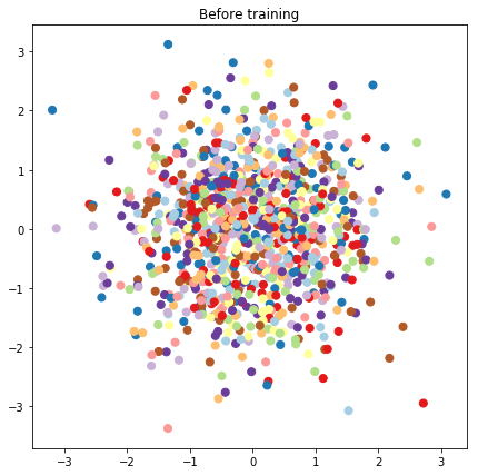
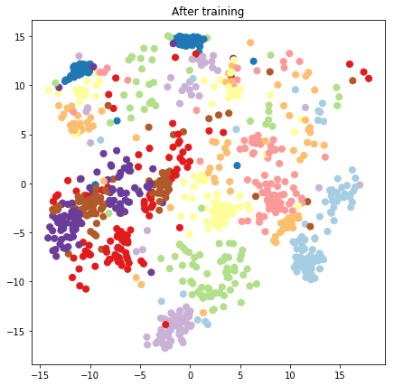
# Plot the latent locations before and after training
plt.figure(figsize=(7, 7))
plt.title("Before training")
plt.grid(False)
plt.scatter(x=init_[:, 0], y=init_[:, 1],
           c=y_train[:N], cmap=plt.get_cmap('Paired'), s=50)
plt.show()

plt.figure(figsize=(7, 7))
plt.title("After training")
plt.grid(False)
plt.scatter(x=lips[-1, :, 0], y=lips[-1, :, 1],
           c=y_train[:N], cmap=plt.get_cmap('Paired'), s=50)
plt.show()
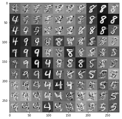
Construct predictive model and sampling ops
# We'll draw samples at evenly spaced points on a 10x10 grid in the latent
# input space.
sample_grid_points = 10
grid_ = np.linspace(-4, 4, sample_grid_points).astype(np.float64)
# Create a 10x10 grid of 2-vectors, for a total shape [10, 10, 2]
grid_ = np.stack(np.meshgrid(grid_, grid_), axis=-1)

# This part's a bit subtle! What we defined above was a batch of 784 (=28x28)
# independent GP distributions over the input space. Each one corresponds to a
# single pixel of an MNIST image. Now what we'd like to do is draw 100 (=10x10)
# *independent* samples, each one separately conditioned on all the observations
# as well as the learned latent input locations above.
#
# The GP regression model below will define a batch of 784 independent
# posteriors. We'd like to get 100 independent samples each at a different
# latent index point. We could loop over the points in the grid, but that might
# be a bit slow. Instead, we can vectorize the computation by tacking on *even
# more* batch dimensions to our GaussianProcessRegressionModel distribution.
# In the below grid_ shape, we have concatentaed
#   1. batch shape: [sample_grid_points, sample_grid_points, 1]
#   2. number of examples: [1]
#   3. number of latent input dimensions: [2]
# The `1` in the batch shape will broadcast with 784. The final result will be
# samples of shape [10, 10, 784, 1]. The `1` comes from the "number of examples"
# and we can just `np.squeeze` it off.
grid_ = grid_.reshape(sample_grid_points, sample_grid_points, 1, 1, 2)

# Create the GPRegressionModel instance which represents the posterior
# predictive at the grid of new points.
gprm = tfd.GaussianProcessRegressionModel(
    kernel=create_kernel(),
    # Shape [10, 10, 1, 1, 2]
    index_points=grid_,
    # Shape [1000, 2]. 1000 2 dimensional vectors.
    observation_index_points=latent_index_points,
    # Shape [784, 1000]. A batch of 784 1000-dimensional observations.
    observations=observations_)
Draw samples conditioned on the data and latent embeddings
We sample at 100 points on a 2-d grid in the latent space.
samples = gprm.sample()

# Plot the grid of samples at new points. We do a bit of tweaking of the samples
# first, squeezing off extra 1-shapes and normalizing the values.
samples_ = np.squeeze(samples.numpy())
samples_ = ((samples_ -
             samples_.min(-1, keepdims=True)) /
            (samples_.max(-1, keepdims=True) -
             samples_.min(-1, keepdims=True)))
samples_ = samples_.reshape(sample_grid_points, sample_grid_points, 28, 28)
samples_ = samples_.transpose([0, 2, 1, 3])
samples_ = samples_.reshape(28 * sample_grid_points, 28 * sample_grid_points)
plt.figure(figsize=(7, 7))
ax = plt.subplot()
ax.grid(False)
ax.imshow(-samples_, interpolation='none', cmap='Greys')
plt.show()
Conclusion
We've taken a brief tour of the Gaussian process latent variable model, and shown how we can implement it in just a few lines of TF and TF Probability code.