
|
|
|
 View source on GitHub View source on GitHub
|
|
Probabilistic principal components analysis (PCA) is a dimensionality reduction technique that analyzes data via a lower dimensional latent space (Tipping and Bishop 1999). It is often used when there are missing values in the data or for multidimensional scaling.
Imports
import functools
import warnings

import matplotlib.pyplot as plt
import numpy as np
import seaborn as sns

import tensorflow as tf
import tf_keras
import tensorflow_probability as tfp

from tensorflow_probability import bijectors as tfb
from tensorflow_probability import distributions as tfd

plt.style.use("ggplot")
warnings.filterwarnings('ignore')
The Model
Consider a data set \(\mathbf{X} = \{\mathbf{x}_n\}\) of \(N\) data points, where each data point is \(D\)-dimensional, $\mathbf{x}_n \in \mathbb{R}^D\(. We aim to represent each \)\mathbf{x}_n$ under a latent variable \(\mathbf{z}_n \in \mathbb{R}^K\) with lower dimension, $K < D\(. The set of principal axes \)\mathbf{W}$ relates the latent variables to the data.
Specifically, we assume that each latent variable is normally distributed,
\[ \begin{equation*} \mathbf{z}_n \sim N(\mathbf{0}, \mathbf{I}). \end{equation*} \]
The corresponding data point is generated via a projection,
\[ \begin{equation*} \mathbf{x}_n \mid \mathbf{z}_n \sim N(\mathbf{W}\mathbf{z}_n, \sigma^2\mathbf{I}), \end{equation*} \]
where the matrix \(\mathbf{W}\in\mathbb{R}^{D\times K}\) are known as the principal axes. In probabilistic PCA, we are typically interested in estimating the principal axes \(\mathbf{W}\) and the noise term \(\sigma^2\).
Probabilistic PCA generalizes classical PCA. Marginalizing out the the latent variable, the distribution of each data point is
\[ \begin{equation*} \mathbf{x}_n \sim N(\mathbf{0}, \mathbf{W}\mathbf{W}^\top + \sigma^2\mathbf{I}). \end{equation*} \]
Classical PCA is the specific case of probabilistic PCA when the covariance of the noise becomes infinitesimally small, \(\sigma^2 \to 0\).
We set up our model below. In our analysis, we assume \(\sigma\) is known, and instead of point estimating \(\mathbf{W}\) as a model parameter, we place a prior over it in order to infer a distribution over principal axes. We'll express the model as a TFP JointDistribution, specifically, we'll use JointDistributionCoroutineAutoBatched.
def probabilistic_pca(data_dim, latent_dim, num_datapoints, stddv_datapoints):
  w = yield tfd.Normal(loc=tf.zeros([data_dim, latent_dim]),
                 scale=2.0 * tf.ones([data_dim, latent_dim]),
                 name="w")
  z = yield tfd.Normal(loc=tf.zeros([latent_dim, num_datapoints]),
                 scale=tf.ones([latent_dim, num_datapoints]),
                 name="z")
  x = yield tfd.Normal(loc=tf.matmul(w, z),
                       scale=stddv_datapoints,
                       name="x")
num_datapoints = 5000
data_dim = 2
latent_dim = 1
stddv_datapoints = 0.5

concrete_ppca_model = functools.partial(probabilistic_pca,
    data_dim=data_dim,
    latent_dim=latent_dim,
    num_datapoints=num_datapoints,
    stddv_datapoints=stddv_datapoints)

model = tfd.JointDistributionCoroutineAutoBatched(concrete_ppca_model)
The Data
We can use the model to generate data by sampling from the joint prior distribution.
actual_w, actual_z, x_train = model.sample()

print("Principal axes:")
print(actual_w)
Principal axes:
tf.Tensor(
[[ 2.2801023]
 [-1.1619819]], shape=(2, 1), dtype=float32)
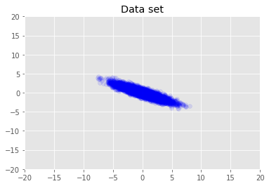
We visualize the dataset.
plt.scatter(x_train[0, :], x_train[1, :], color='blue', alpha=0.1)
plt.axis([-20, 20, -20, 20])
plt.title("Data set")
plt.show()
Maximum a Posteriori Inference
We first search for the point estimate of latent variables that maximizes the posterior probability density. This is known as maximum a posteriori (MAP) inference, and is done by calculating the values of \(\mathbf{W}\) and \(\mathbf{Z}\) that maximise the posterior density \(p(\mathbf{W}, \mathbf{Z} \mid \mathbf{X}) \propto p(\mathbf{W}, \mathbf{Z}, \mathbf{X})\).
w = tf.Variable(tf.random.normal([data_dim, latent_dim]))
z = tf.Variable(tf.random.normal([latent_dim, num_datapoints]))
target_log_prob_fn = lambda w, z: model.log_prob((w, z, x_train))
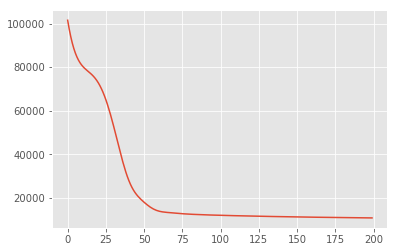
losses = tfp.math.minimize(
lambda: -target_log_prob_fn(w, z),
optimizer=tf_keras.optimizers.Adam(learning_rate=0.05),
num_steps=200)
plt.plot(losses)
[<matplotlib.lines.Line2D at 0x7f19897a42e8>]
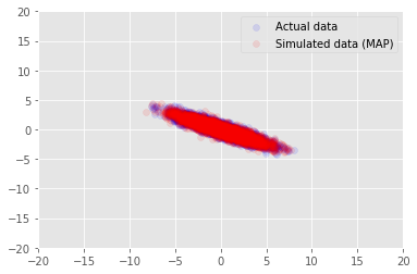
We can use the model to sample data for the inferred values for \(\mathbf{W}\) and \(\mathbf{Z}\), and compare to the actual dataset we conditioned on.
print("MAP-estimated axes:")
print(w)

_, _, x_generated = model.sample(value=(w, z, None))

plt.scatter(x_train[0, :], x_train[1, :], color='blue', alpha=0.1, label='Actual data')
plt.scatter(x_generated[0, :], x_generated[1, :], color='red', alpha=0.1, label='Simulated data (MAP)')
plt.legend()
plt.axis([-20, 20, -20, 20])
plt.show()
MAP-estimated axes:
<tf.Variable 'Variable:0' shape=(2, 1) dtype=float32, numpy=
array([[ 2.9135954],
       [-1.4826864]], dtype=float32)>
Variational Inference
MAP can be used to find the mode (or one of the modes) of the posterior distribution, but does not provide any other insights about it. We next use variational inference, where the posterior distribtion \(p(\mathbf{W}, \mathbf{Z} \mid \mathbf{X})\) is approximated using a variational distribution \(q(\mathbf{W}, \mathbf{Z})\) parametrised by \(\boldsymbol{\lambda}\). The aim is to find the variational parameters \(\boldsymbol{\lambda}\) that minimize the KL divergence between q and the posterior, \(\mathrm{KL}(q(\mathbf{W}, \mathbf{Z}) \mid\mid p(\mathbf{W}, \mathbf{Z} \mid \mathbf{X}))\), or equivalently, that maximize the evidence lower bound, \(\mathbb{E}_{q(\mathbf{W},\mathbf{Z};\boldsymbol{\lambda})}\left[ \log p(\mathbf{W},\mathbf{Z},\mathbf{X}) - \log q(\mathbf{W},\mathbf{Z}; \boldsymbol{\lambda}) \right]\).
qw_mean = tf.Variable(tf.random.normal([data_dim, latent_dim]))
qz_mean = tf.Variable(tf.random.normal([latent_dim, num_datapoints]))
qw_stddv = tfp.util.TransformedVariable(1e-4 * tf.ones([data_dim, latent_dim]),
bijector=tfb.Softplus())
qz_stddv = tfp.util.TransformedVariable(
1e-4 * tf.ones([latent_dim, num_datapoints]),
bijector=tfb.Softplus())
def factored_normal_variational_model():
qw = yield tfd.Normal(loc=qw_mean, scale=qw_stddv, name="qw")
qz = yield tfd.Normal(loc=qz_mean, scale=qz_stddv, name="qz")
surrogate_posterior = tfd.JointDistributionCoroutineAutoBatched(
factored_normal_variational_model)
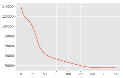
losses = tfp.vi.fit_surrogate_posterior(
target_log_prob_fn,
surrogate_posterior=surrogate_posterior,
optimizer=tf_keras.optimizers.Adam(learning_rate=0.05),
num_steps=200)
print("Inferred axes:")
print(qw_mean)
print("Standard Deviation:")
print(qw_stddv)

plt.plot(losses)
plt.show()
Inferred axes:
<tf.Variable 'Variable:0' shape=(2, 1) dtype=float32, numpy=
array([[ 2.4168603],
       [-1.2236133]], dtype=float32)>
Standard Deviation:
<TransformedVariable: dtype=float32, shape=[2, 1], fn="softplus", numpy=
array([[0.0042499 ],
       [0.00598824]], dtype=float32)>
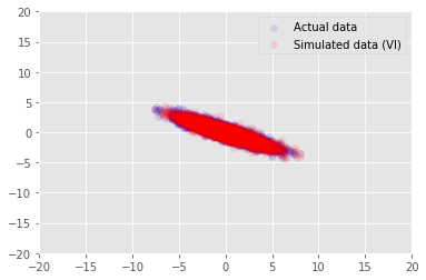
posterior_samples = surrogate_posterior.sample(50)
_, _, x_generated = model.sample(value=(posterior_samples))

# It's a pain to plot all 5000 points for each of our 50 posterior samples, so
# let's subsample to get the gist of the distribution.
x_generated = tf.reshape(tf.transpose(x_generated, [1, 0, 2]), (2, -1))[:, ::47]

plt.scatter(x_train[0, :], x_train[1, :], color='blue', alpha=0.1, label='Actual data')
plt.scatter(x_generated[0, :], x_generated[1, :], color='red', alpha=0.1, label='Simulated data (VI)')
plt.legend()
plt.axis([-20, 20, -20, 20])
plt.show()
Acknowledgements
This tutorial was originally written in Edward 1.0 (source). We thank all contributors to writing and revising that version.
References
[1]: Michael E. Tipping and Christopher M. Bishop. Probabilistic principal component analysis. Journal of the Royal Statistical Society: Series B (Statistical Methodology), 61(3): 611-622, 1999.