
| |  GitHubでソースを表示 GitHubでソースを表示 | |
このチュートリアルでは、量子回路の期待値の勾配計算アルゴリズムについて説明します。
量子回路で観測可能な特定の期待値の勾配を計算することは、複雑なプロセスです。観測可能な値の期待値には、書き留めるのが簡単な分析勾配式を持つ従来の機械学習変換とは異なり、常に書き留めるのが簡単な分析勾配式を持つという贅沢はありません。その結果、さまざまなシナリオで役立つさまざまな量子勾配計算方法があります。このチュートリアルでは、2つの異なる微分スキームを比較対照します。
設定
pip install tensorflow==2.7.0
TensorFlowQuantumをインストールします。
pip install tensorflow-quantum
# Update package resources to account for version changes.
import importlib, pkg_resources
importlib.reload(pkg_resources)
<module 'pkg_resources' from '/tmpfs/src/tf_docs_env/lib/python3.7/site-packages/pkg_resources/__init__.py'>
次に、TensorFlowとモジュールの依存関係をインポートします。
import tensorflow as tf
import tensorflow_quantum as tfq

import cirq
import sympy
import numpy as np

# visualization tools
%matplotlib inline
import matplotlib.pyplot as plt
from cirq.contrib.svg import SVGCircuit
2022-02-04 12:25:24.733670: E tensorflow/stream_executor/cuda/cuda_driver.cc:271] failed call to cuInit: CUDA_ERROR_NO_DEVICE: no CUDA-capable device is detectedプレースホルダー19
1.予備
量子回路の勾配計算の概念をもう少し具体的にしましょう。次のようなパラメータ化された回路があるとします。
qubit = cirq.GridQubit(0, 0)
my_circuit = cirq.Circuit(cirq.Y(qubit)**sympy.Symbol('alpha'))
SVGCircuit(my_circuit)
findfont: Font family ['Arial'] not found. Falling back to DejaVu Sans.

オブザーバブルとともに:
pauli_x = cirq.X(qubit)
pauli_x
cirq.X(cirq.GridQubit(0, 0))
この演算子を見ると、 \(⟨Y(\alpha)| X | Y(\alpha)⟩ = \sin(\pi \alpha)\)であることがわかります。
def my_expectation(op, alpha):
    """Compute ⟨Y(alpha)| `op` | Y(alpha)⟩"""
    params = {'alpha': alpha}
    sim = cirq.Simulator()
    final_state_vector = sim.simulate(my_circuit, params).final_state_vector
    return op.expectation_from_state_vector(final_state_vector, {qubit: 0}).real


my_alpha = 0.3
print("Expectation=", my_expectation(pauli_x, my_alpha))
print("Sin Formula=", np.sin(np.pi * my_alpha))
Expectation= 0.80901700258255
Sin Formula= 0.8090169943749475
また、 \(f_{1}(\alpha) = ⟨Y(\alpha)| X | Y(\alpha)⟩\) を定義すると、 \(f_{1}^{'}(\alpha) = \pi \cos(\pi \alpha)\)になります。これを確認しましょう:
def my_grad(obs, alpha, eps=0.01):
    grad = 0
    f_x = my_expectation(obs, alpha)
    f_x_prime = my_expectation(obs, alpha + eps)
    return ((f_x_prime - f_x) / eps).real


print('Finite difference:', my_grad(pauli_x, my_alpha))
print('Cosine formula:   ', np.pi * np.cos(np.pi * my_alpha))
Finite difference: 1.8063604831695557
Cosine formula:    1.8465818304904567
プレースホルダー27
2.差別化要因の必要性
より大きな回路では、与えられた量子回路の勾配を正確に計算する式を持っていることは必ずしも幸運ではありません。勾配を計算するには単純な式では不十分な場合、 tfq.differentiators.Differentiatorクラスを使用すると、回路の勾配を計算するためのアルゴリズムを定義できます。たとえば、TensorFlow Quantum(TFQ)で上記の例を次のように再現できます。
expectation_calculation = tfq.layers.Expectation(
    differentiator=tfq.differentiators.ForwardDifference(grid_spacing=0.01))

expectation_calculation(my_circuit,
                        operators=pauli_x,
                        symbol_names=['alpha'],
                        symbol_values=[[my_alpha]])
<tf.Tensor: shape=(1, 1), dtype=float32, numpy=array([[0.80901706]], dtype=float32)>プレースホルダー29
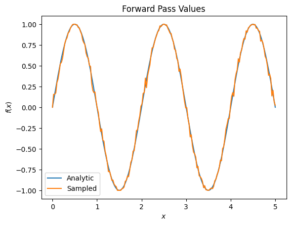
ただし、サンプリング(実際のデバイスで何が起こるか)に基づいて期待値を推定するように切り替えると、値が少し変わる可能性があります。これは、見積もりが不完全であることを意味します。
sampled_expectation_calculation = tfq.layers.SampledExpectation(
    differentiator=tfq.differentiators.ForwardDifference(grid_spacing=0.01))

sampled_expectation_calculation(my_circuit,
                                operators=pauli_x,
                                repetitions=500,
                                symbol_names=['alpha'],
                                symbol_values=[[my_alpha]])
<tf.Tensor: shape=(1, 1), dtype=float32, numpy=array([[0.836]], dtype=float32)>
これは、勾配に関しては、すぐに深刻な精度の問題に発展する可能性があります。
# Make input_points = [batch_size, 1] array.
input_points = np.linspace(0, 5, 200)[:, np.newaxis].astype(np.float32)
exact_outputs = expectation_calculation(my_circuit,
                                        operators=pauli_x,
                                        symbol_names=['alpha'],
                                        symbol_values=input_points)
imperfect_outputs = sampled_expectation_calculation(my_circuit,
                                                    operators=pauli_x,
                                                    repetitions=500,
                                                    symbol_names=['alpha'],
                                                    symbol_values=input_points)
plt.title('Forward Pass Values')
plt.xlabel('$x$')
plt.ylabel('$f(x)$')
plt.plot(input_points, exact_outputs, label='Analytic')
plt.plot(input_points, imperfect_outputs, label='Sampled')
plt.legend()
<matplotlib.legend.Legend at 0x7ff07d556190>
# Gradients are a much different story.
values_tensor = tf.convert_to_tensor(input_points)

with tf.GradientTape() as g:
    g.watch(values_tensor)
    exact_outputs = expectation_calculation(my_circuit,
                                            operators=pauli_x,
                                            symbol_names=['alpha'],
                                            symbol_values=values_tensor)
analytic_finite_diff_gradients = g.gradient(exact_outputs, values_tensor)

with tf.GradientTape() as g:
    g.watch(values_tensor)
    imperfect_outputs = sampled_expectation_calculation(
        my_circuit,
        operators=pauli_x,
        repetitions=500,
        symbol_names=['alpha'],
        symbol_values=values_tensor)
sampled_finite_diff_gradients = g.gradient(imperfect_outputs, values_tensor)

plt.title('Gradient Values')
plt.xlabel('$x$')
plt.ylabel('$f^{\'}(x)$')
plt.plot(input_points, analytic_finite_diff_gradients, label='Analytic')
plt.plot(input_points, sampled_finite_diff_gradients, label='Sampled')
plt.legend()
<matplotlib.legend.Legend at 0x7ff07adb8dd0>
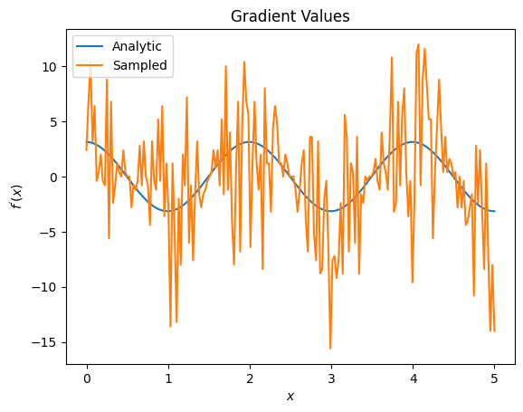
ここで、分析の場合、有限差分式自体は勾配自体を計算するのに高速ですが、サンプリングベースの方法に関しては、ノイズが多すぎることがわかります。良好な勾配を確実に計算するには、より注意深い手法を使用する必要があります。次に、分析的期待勾配計算にはあまり適していないが、実際のサンプルベースのケースでははるかに優れたパフォーマンスを発揮する、はるかに遅い手法を見ていきます。
# A smarter differentiation scheme.
gradient_safe_sampled_expectation = tfq.layers.SampledExpectation(
    differentiator=tfq.differentiators.ParameterShift())

with tf.GradientTape() as g:
    g.watch(values_tensor)
    imperfect_outputs = gradient_safe_sampled_expectation(
        my_circuit,
        operators=pauli_x,
        repetitions=500,
        symbol_names=['alpha'],
        symbol_values=values_tensor)

sampled_param_shift_gradients = g.gradient(imperfect_outputs, values_tensor)

plt.title('Gradient Values')
plt.xlabel('$x$')
plt.ylabel('$f^{\'}(x)$')
plt.plot(input_points, analytic_finite_diff_gradients, label='Analytic')
plt.plot(input_points, sampled_param_shift_gradients, label='Sampled')
plt.legend()
<matplotlib.legend.Legend at 0x7ff07ad9ff90>
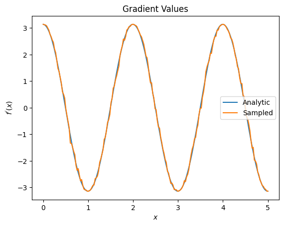
上記から、特定の研究シナリオに特定の差別化要因が最適に使用されていることがわかります。一般に、デバイスノイズなどに対して堅牢な、より低速なサンプルベースの方法は、より「現実の」設定でアルゴリズムをテストまたは実装する場合の大きな差別化要因です。有限差分などのより高速な方法は分析計算に最適であり、より高いスループットが必要ですが、アルゴリズムのデバイスの実行可能性にはまだ関心がありません。
3.複数のオブザーバブル
2番目のオブザーバブルを紹介し、TensorFlowQuantumが単一の回路に対して複数のオブザーバブルをサポートする方法を見てみましょう。
pauli_z = cirq.Z(qubit)
pauli_z
cirq.Z(cirq.GridQubit(0, 0))
このオブザーバブルが以前と同じ回路で使用されている場合、 \(f_{2}(\alpha) = ⟨Y(\alpha)| Z | Y(\alpha)⟩ = \cos(\pi \alpha)\) と \(f_{2}^{'}(\alpha) = -\pi \sin(\pi \alpha)\)があります。クイックチェックを実行します。
test_value = 0.

print('Finite difference:', my_grad(pauli_z, test_value))
print('Sin formula:      ', -np.pi * np.sin(np.pi * test_value))
Finite difference: -0.04934072494506836
Sin formula:       -0.0
それは一致です(十分に近い)。
ここで、 \(g(\alpha) = f_{1}(\alpha) + f_{2}(\alpha)\) \(g'(\alpha) = f_{1}^{'}(\alpha) + f^{'}_{2}(\alpha)\)なります。 TensorFlow Quantumで複数のオブザーバブルを定義して回路と一緒に使用することは、 \(g\)にさらに用語を追加することと同じです。
これは、回路内の特定のシンボルの勾配が、その回路に適用されたそのシンボルについて観測可能な各シンボルに関する勾配の合計に等しいことを意味します。これは、TensorFlowの勾配取得およびバックプロパゲーション(特定のシンボルの勾配としてすべてのオブザーバブルの勾配の合計を指定する)と互換性があります。
sum_of_outputs = tfq.layers.Expectation(
    differentiator=tfq.differentiators.ForwardDifference(grid_spacing=0.01))

sum_of_outputs(my_circuit,
               operators=[pauli_x, pauli_z],
               symbol_names=['alpha'],
               symbol_values=[[test_value]])
<tf.Tensor: shape=(1, 2), dtype=float32, numpy=array([[1.9106855e-15, 1.0000000e+00]], dtype=float32)>
ここで、最初のエントリはPauli Xの期待値であり、2番目のエントリはPauliZの期待値です。勾配をとると次のようになります。
test_value_tensor = tf.convert_to_tensor([[test_value]])

with tf.GradientTape() as g:
    g.watch(test_value_tensor)
    outputs = sum_of_outputs(my_circuit,
                             operators=[pauli_x, pauli_z],
                             symbol_names=['alpha'],
                             symbol_values=test_value_tensor)

sum_of_gradients = g.gradient(outputs, test_value_tensor)

print(my_grad(pauli_x, test_value) + my_grad(pauli_z, test_value))
print(sum_of_gradients.numpy())
3.0917350202798843
[[3.0917213]]
ここで、各オブザーバブルの勾配の合計が実際に \(\alpha\)の勾配であることを確認しました。この動作は、すべてのTensorFlow Quantum微分器によってサポートされており、残りのTensorFlowとの互換性において重要な役割を果たします。
4.高度な使用法
TensorFlowQuantumサブクラスtfq.differentiators.Differentiator内に存在するすべての微分器。差別化要因を実装するには、ユーザーは2つのインターフェースのいずれかを実装する必要があります。標準はget_gradient_circuitsを実装することです。これは、勾配の推定値を取得するために測定する回路を基本クラスに指示します。または、 differentiate_analyticとdifferentiate_sampledをオーバーロードすることもできます。クラスtfq.differentiators.Adjointはこのルートを取ります。
以下では、TensorFlow Quantumを使用して、回路の勾配を実装しています。パラメータシフトの小さな例を使用します。
上で定義した回路、 \(|\alpha⟩ = Y^{\alpha}|0⟩\)を思い出してください。前と同じように、 \(X\) observable、 \(f(\alpha) = ⟨\alpha|X|\alpha⟩\)placeholder12に対するこの回路の期待値として関数を定義できます。パラメータシフトルールを使用すると、この回路の導関数は次のようになります。
\[\frac{\partial}{\partial \alpha} f(\alpha) = \frac{\pi}{2} f\left(\alpha + \frac{1}{2}\right) - \frac{ \pi}{2} f\left(\alpha - \frac{1}{2}\right)\]
get_gradient_circuits関数は、この導関数のコンポーネントを返します。
class MyDifferentiator(tfq.differentiators.Differentiator):
    """A Toy differentiator for <Y^alpha | X |Y^alpha>."""

    def __init__(self):
        pass

    def get_gradient_circuits(self, programs, symbol_names, symbol_values):
        """Return circuits to compute gradients for given forward pass circuits.

        Every gradient on a quantum computer can be computed via measurements
        of transformed quantum circuits.  Here, you implement a custom gradient
        for a specific circuit.  For a real differentiator, you will need to
        implement this function in a more general way.  See the differentiator
        implementations in the TFQ library for examples.
        """

        # The two terms in the derivative are the same circuit...
        batch_programs = tf.stack([programs, programs], axis=1)

        # ... with shifted parameter values.
        shift = tf.constant(1/2)
        forward = symbol_values + shift
        backward = symbol_values - shift
        batch_symbol_values = tf.stack([forward, backward], axis=1)

        # Weights are the coefficients of the terms in the derivative.
        num_program_copies = tf.shape(batch_programs)[0]
        batch_weights = tf.tile(tf.constant([[[np.pi/2, -np.pi/2]]]),
                                [num_program_copies, 1, 1])

        # The index map simply says which weights go with which circuits.
        batch_mapper = tf.tile(
            tf.constant([[[0, 1]]]), [num_program_copies, 1, 1])

        return (batch_programs, symbol_names, batch_symbol_values,
                batch_weights, batch_mapper)
Differentiator器の基本クラスは、上記のパラメーターシフト式のように、 get_gradient_circuitsから返されたコンポーネントを使用して導関数を計算します。この新しい差別化要因は、既存のtfq.layerオブジェクトで使用できるようになりました。
custom_dif = MyDifferentiator()
custom_grad_expectation = tfq.layers.Expectation(differentiator=custom_dif)

# Now let's get the gradients with finite diff.
with tf.GradientTape() as g:
    g.watch(values_tensor)
    exact_outputs = expectation_calculation(my_circuit,
                                            operators=[pauli_x],
                                            symbol_names=['alpha'],
                                            symbol_values=values_tensor)

analytic_finite_diff_gradients = g.gradient(exact_outputs, values_tensor)

# Now let's get the gradients with custom diff.
with tf.GradientTape() as g:
    g.watch(values_tensor)
    my_outputs = custom_grad_expectation(my_circuit,
                                         operators=[pauli_x],
                                         symbol_names=['alpha'],
                                         symbol_values=values_tensor)

my_gradients = g.gradient(my_outputs, values_tensor)

plt.subplot(1, 2, 1)
plt.title('Exact Gradient')
plt.plot(input_points, analytic_finite_diff_gradients.numpy())
plt.xlabel('x')
plt.ylabel('f(x)')
plt.subplot(1, 2, 2)
plt.title('My Gradient')
plt.plot(input_points, my_gradients.numpy())
plt.xlabel('x')
Text(0.5, 0, 'x')
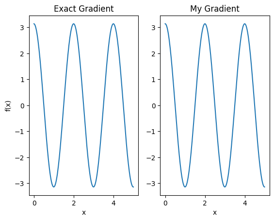
この新しい微分器を使用して、微分可能な演算を生成できるようになりました。
# Create a noisy sample based expectation op.
expectation_sampled = tfq.get_sampled_expectation_op(
    cirq.DensityMatrixSimulator(noise=cirq.depolarize(0.01)))

# Make it differentiable with your differentiator:
# Remember to refresh the differentiator before attaching the new op
custom_dif.refresh()
differentiable_op = custom_dif.generate_differentiable_op(
    sampled_op=expectation_sampled)

# Prep op inputs.
circuit_tensor = tfq.convert_to_tensor([my_circuit])
op_tensor = tfq.convert_to_tensor([[pauli_x]])
single_value = tf.convert_to_tensor([[my_alpha]])
num_samples_tensor = tf.convert_to_tensor([[5000]])

with tf.GradientTape() as g:
    g.watch(single_value)
    forward_output = differentiable_op(circuit_tensor, ['alpha'], single_value,
                                       op_tensor, num_samples_tensor)

my_gradients = g.gradient(forward_output, single_value)

print('---TFQ---')
print('Foward:  ', forward_output.numpy())
print('Gradient:', my_gradients.numpy())
print('---Original---')
print('Forward: ', my_expectation(pauli_x, my_alpha))
print('Gradient:', my_grad(pauli_x, my_alpha))
---TFQ---
Foward:   [[0.8016]]
Gradient: [[1.7932211]]
---Original---
Forward:  0.80901700258255
Gradient: 1.8063604831695557