
| | |  GitHub पर स्रोत देखें GitHub पर स्रोत देखें | |
यह ट्यूटोरियल दिखाता है कि कैसे एक शास्त्रीय तंत्रिका नेटवर्क qubit अंशांकन त्रुटियों को ठीक करना सीख सकता है। यह शोर इंटरमीडिएट स्केल क्वांटम (एनआईएसक्यू) सर्किट बनाने, संपादित करने और आह्वान करने के लिए एक पायथन फ्रेमवर्क सर्क पेश करता है, और दर्शाता है कि सर्क टेन्सरफ्लो क्वांटम के साथ कैसे इंटरफेस करता है।
सेट अप
pip install tensorflow==2.7.0
TensorFlow क्वांटम स्थापित करें:
pip install tensorflow-quantum
# Update package resources to account for version changes.
import importlib, pkg_resources
importlib.reload(pkg_resources)
<module 'pkg_resources' from '/tmpfs/src/tf_docs_env/lib/python3.7/site-packages/pkg_resources/__init__.py'>
अब TensorFlow और मॉड्यूल निर्भरताएँ आयात करें:
import tensorflow as tf
import tensorflow_quantum as tfq

import cirq
import sympy
import numpy as np

# visualization tools
%matplotlib inline
import matplotlib.pyplot as plt
from cirq.contrib.svg import SVGCircuit
2022-02-04 12:27:31.677071: E tensorflow/stream_executor/cuda/cuda_driver.cc:271] failed call to cuInit: CUDA_ERROR_NO_DEVICE: no CUDA-capable device is detectedप्लेसहोल्डर17
1. मूल बातें
1.1 सर्क और पैरामीटरयुक्त क्वांटम सर्किट
TensorFlow क्वांटम (TFQ) की खोज करने से पहले, आइए कुछ Cirq मूल बातें देखें। Cirq Google की ओर से क्वांटम कंप्यूटिंग के लिए एक पायथन लाइब्रेरी है। आप इसका उपयोग सर्किट को परिभाषित करने के लिए करते हैं, जिसमें स्थिर और पैरामीटरयुक्त गेट शामिल हैं।
Cirq मुक्त मापदंडों का प्रतिनिधित्व करने के लिए SymPy प्रतीकों का उपयोग करता है।
a, b = sympy.symbols('a b')
निम्नलिखित कोड आपके मापदंडों का उपयोग करके दो-क्विट सर्किट बनाता है:
# Create two qubits
q0, q1 = cirq.GridQubit.rect(1, 2)

# Create a circuit on these qubits using the parameters you created above.
circuit = cirq.Circuit(
    cirq.rx(a).on(q0),
    cirq.ry(b).on(q1), cirq.CNOT(control=q0, target=q1))

SVGCircuit(circuit)
findfont: Font family ['Arial'] not found. Falling back to DejaVu Sans.

सर्किट का मूल्यांकन करने के लिए, आप cirq.Simulator इंटरफ़ेस का उपयोग कर सकते हैं। आप एक सर्किट में मुफ्त पैरामीटर को विशिष्ट संख्याओं के साथ एक cirq.ParamResolver ऑब्जेक्ट में पास करके प्रतिस्थापित करते हैं। निम्नलिखित कोड आपके पैरामीटरयुक्त सर्किट के कच्चे राज्य वेक्टर आउटपुट की गणना करता है:
# Calculate a state vector with a=0.5 and b=-0.5.
resolver = cirq.ParamResolver({a: 0.5, b: -0.5})
output_state_vector = cirq.Simulator().simulate(circuit, resolver).final_state_vector
output_state_vector
array([ 0.9387913 +0.j        , -0.23971277+0.j        ,

        0.        +0.06120872j,  0.        -0.23971277j], dtype=complex64)
प्लेसहोल्डर22सिमुलेशन के बाहर राज्य वैक्टर सीधे पहुंच योग्य नहीं हैं (उपरोक्त आउटपुट में जटिल संख्याओं पर ध्यान दें)। भौतिक रूप से यथार्थवादी होने के लिए, आपको एक माप निर्दिष्ट करना होगा, जो एक राज्य वेक्टर को एक वास्तविक संख्या में परिवर्तित करता है जिसे शास्त्रीय कंप्यूटर समझ सकते हैं। Cirq पाउली ऑपरेटरों \(\hat{X}\), \(\hat{Y}\), और \(\hat{Z}\)के संयोजन का उपयोग करके माप निर्दिष्ट करता है। उदाहरण के तौर पर, निम्न कोड आपके द्वारा अनुकरण किए गए राज्य वेक्टर पर l10n \(\hat{Z}_0\) और \(\frac{1}{2}\hat{Z}_0 + \hat{X}_1\) को मापता है:
z0 = cirq.Z(q0)

qubit_map={q0: 0, q1: 1}

z0.expectation_from_state_vector(output_state_vector, qubit_map).real
0.8775825500488281
z0x1 = 0.5 * z0 + cirq.X(q1)

z0x1.expectation_from_state_vector(output_state_vector, qubit_map).real
-0.04063427448272705
1.2 क्वांटम सर्किट टेंसर के रूप में
TensorFlow क्वांटम (TFQ) tfq.convert_to_tensor प्रदान करता है, एक फ़ंक्शन जो Cirq ऑब्जेक्ट को टेंसर में परिवर्तित करता है। यह आपको हमारे क्वांटम लेयर्स और क्वांटम ऑप्स में Cirq ऑब्जेक्ट भेजने की अनुमति देता है। फ़ंक्शन को Cirq सर्किट और Cirq Paulis की सूचियों या सरणियों पर बुलाया जा सकता है:
# Rank 1 tensor containing 1 circuit.
circuit_tensor = tfq.convert_to_tensor([circuit])

print(circuit_tensor.shape)
print(circuit_tensor.dtype)
(1,)
<dtype: 'string'>
यह सर्क ऑब्जेक्ट्स को tf.string टेंसर के रूप में एन्कोड करता है जो tfq ऑपरेशंस आवश्यकतानुसार डीकोड करता है।
# Rank 1 tensor containing 2 Pauli operators.
pauli_tensor = tfq.convert_to_tensor([z0, z0x1])
pauli_tensor.shape
TensorShape([2])
1.3 बैचिंग सर्किट सिमुलेशन
TFQ अपेक्षा मूल्यों, नमूनों और राज्य वैक्टर की गणना के लिए तरीके प्रदान करता है। अभी के लिए, आइए उम्मीद के मूल्यों पर ध्यान दें।
अपेक्षा मूल्यों की गणना के लिए उच्चतम-स्तरीय इंटरफ़ेस tfq.layers.Expectation परत है, जो एक tf.keras.Layer है। अपने सरलतम रूप में, यह परत कई सर्किल पर एक पैरामीटरयुक्त सर्किट को अनुकरण करने के बराबर है। cirq.ParamResolvers ; हालांकि, TFQ TensorFlow सेमेन्टिक्स के बाद बैचिंग की अनुमति देता है, और सर्किट को कुशल C++ कोड का उपयोग करके सिम्युलेटेड किया जाता है।
हमारे a और b पैरामीटर के स्थानापन्न के लिए मानों का एक बैच बनाएं:
batch_vals = np.array(np.random.uniform(0, 2 * np.pi, (5, 2)), dtype=np.float32)
Cirq में पैरामीटर मानों पर सर्किट निष्पादन को बैचने के लिए एक लूप की आवश्यकता होती है:
cirq_results = []
cirq_simulator = cirq.Simulator()

for vals in batch_vals:
    resolver = cirq.ParamResolver({a: vals[0], b: vals[1]})
    final_state_vector = cirq_simulator.simulate(circuit, resolver).final_state_vector
    cirq_results.append(
        [z0.expectation_from_state_vector(final_state_vector, {
            q0: 0,
            q1: 1
        }).real])

print('cirq batch results: \n {}'.format(np.array(cirq_results)))
cirq batch results:
 [[-0.66652703]
 [ 0.49764055]
 [ 0.67326665]
 [-0.95549959]
 [-0.81297827]]
प्लेसहोल्डर33
टीएफक्यू में एक ही ऑपरेशन को सरल बनाया गया है:
tfq.layers.Expectation()(circuit,
                         symbol_names=[a, b],
                         symbol_values=batch_vals,
                         operators=z0)
<tf.Tensor: shape=(5, 1), dtype=float32, numpy=
array([[-0.666526  ],
       [ 0.49764216],
       [ 0.6732664 ],
       [-0.9554999 ],
       [-0.8129788 ]], dtype=float32)>
2. हाइब्रिड क्वांटम-शास्त्रीय अनुकूलन
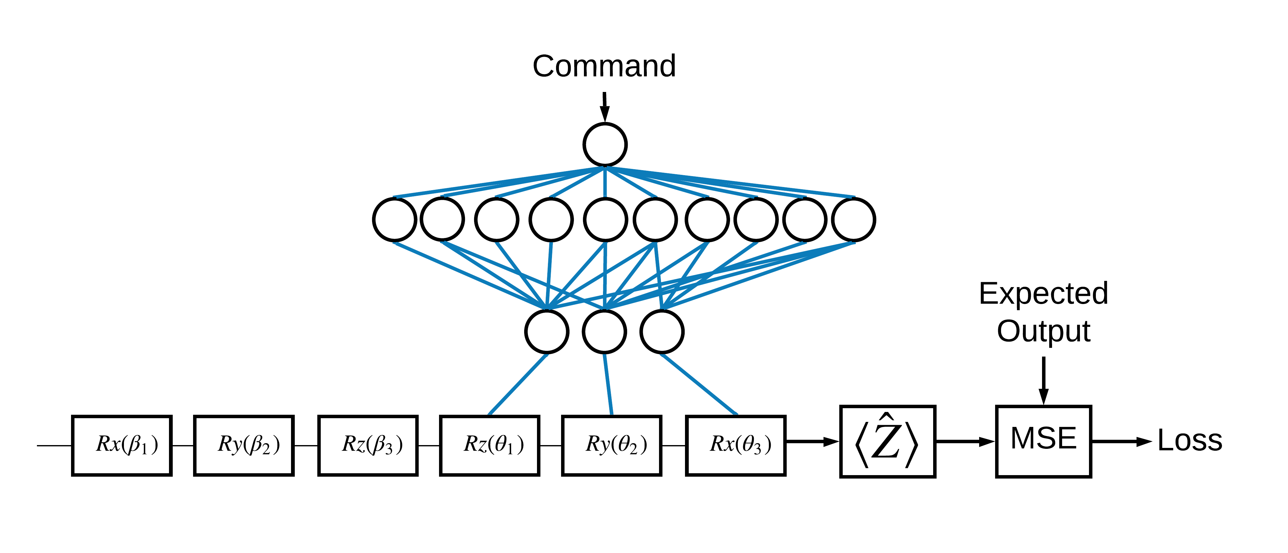
अब जब आपने मूल बातें देख ली हैं, तो चलिए एक हाइब्रिड क्वांटम-क्लासिकल न्यूरल नेट बनाने के लिए TensorFlow क्वांटम का उपयोग करते हैं। आप एक एकल कक्षा को नियंत्रित करने के लिए एक शास्त्रीय तंत्रिका जाल को प्रशिक्षित करेंगे। सिम्युलेटेड व्यवस्थित कैलिब्रेशन त्रुटि पर काबू पाने के लिए नियंत्रण को 0 या 1 अवस्था में qubit को सही ढंग से तैयार करने के लिए अनुकूलित किया जाएगा। यह आंकड़ा वास्तुकला को दर्शाता है:
तंत्रिका नेटवर्क के बिना भी यह हल करने के लिए एक सीधी समस्या है, लेकिन विषय वास्तविक क्वांटम नियंत्रण समस्याओं के समान है जिसे आप TFQ का उपयोग करके हल कर सकते हैं। यह एक tf.keras.Model के अंदर tfq.layers.ControlledPQC (पैरामीट्रिज्ड क्वांटम सर्किट) परत का उपयोग करके क्वांटम-शास्त्रीय गणना का एक एंड-टू-एंड उदाहरण प्रदर्शित करता है।
इस ट्यूटोरियल के कार्यान्वयन के लिए, इस आर्किटेक्चर को 3 भागों में विभाजित किया गया है:
- इनपुट सर्किट या डेटापॉइंट सर्किट : पहले तीन \(R\) गेट।
- नियंत्रित परिपथ : अन्य तीन \(R\) द्वार।
- नियंत्रक : शास्त्रीय तंत्रिका-नेटवर्क नियंत्रित सर्किट के मापदंडों को निर्धारित करता है।
2.1 नियंत्रित सर्किट परिभाषा
एक सीखने योग्य सिंगल बिट रोटेशन को परिभाषित करें, जैसा कि ऊपर की आकृति में दर्शाया गया है। यह हमारे नियंत्रित सर्किट के अनुरूप होगा।
# Parameters that the classical NN will feed values into.
control_params = sympy.symbols('theta_1 theta_2 theta_3')

# Create the parameterized circuit.
qubit = cirq.GridQubit(0, 0)
model_circuit = cirq.Circuit(
    cirq.rz(control_params[0])(qubit),
    cirq.ry(control_params[1])(qubit),
    cirq.rx(control_params[2])(qubit))

SVGCircuit(model_circuit)

2.2 नियंत्रक
अब नियंत्रक नेटवर्क को परिभाषित करें:
# The classical neural network layers.
controller = tf.keras.Sequential([
    tf.keras.layers.Dense(10, activation='elu'),
    tf.keras.layers.Dense(3)
])
आदेशों के एक बैच को देखते हुए, नियंत्रक नियंत्रित सर्किट के लिए नियंत्रण संकेतों के एक बैच को आउटपुट करता है।
नियंत्रक यादृच्छिक रूप से प्रारंभ किया गया है, इसलिए ये आउटपुट उपयोगी नहीं हैं, फिर भी।
controller(tf.constant([[0.0],[1.0]])).numpy()
array([[0.        , 0.        , 0.        ],
       [0.5815686 , 0.21376055, 0.57181627]], dtype=float32)
2.3 नियंत्रक को सर्किट से कनेक्ट करें
नियंत्रक को नियंत्रित सर्किट से जोड़ने के लिए tfq का उपयोग एकल keras.Model के रूप में करें।
मॉडल परिभाषा की इस शैली के बारे में अधिक जानकारी के लिए केरस फंक्शनल एपीआई गाइड देखें।
पहले मॉडल में इनपुट को परिभाषित करें:
# This input is the simulated miscalibration that the model will learn to correct.
circuits_input = tf.keras.Input(shape=(),
                                # The circuit-tensor has dtype `tf.string`
                                dtype=tf.string,
                                name='circuits_input')

# Commands will be either `0` or `1`, specifying the state to set the qubit to.
commands_input = tf.keras.Input(shape=(1,),
                                dtype=tf.dtypes.float32,
                                name='commands_input')
गणना को परिभाषित करने के लिए अगला उन इनपुटों पर संचालन लागू करें।
dense_2 = controller(commands_input)

# TFQ layer for classically controlled circuits.
expectation_layer = tfq.layers.ControlledPQC(model_circuit,
                                             # Observe Z
                                             operators = cirq.Z(qubit))
expectation = expectation_layer([circuits_input, dense_2])
अब इस गणना को tf.keras.Model के रूप में पैकेज करें:
# The full Keras model is built from our layers.
model = tf.keras.Model(inputs=[circuits_input, commands_input],
                       outputs=expectation)
नेटवर्क आर्किटेक्चर को नीचे दिए गए मॉडल के प्लॉट द्वारा दर्शाया गया है। शुद्धता को सत्यापित करने के लिए इस मॉडल प्लॉट की तुलना आर्किटेक्चर आरेख से करें।
tf.keras.utils.plot_model(model, show_shapes=True, dpi=70)
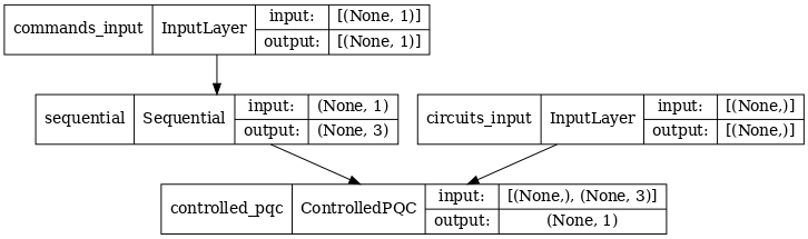
यह मॉडल दो इनपुट लेता है: नियंत्रक के लिए आदेश, और इनपुट-सर्किट जिसका आउटपुट नियंत्रक सही करने का प्रयास कर रहा है।
2.4 डेटासेट
मॉडल प्रत्येक कमांड के लिए \(\hat{Z}\) के सही सही माप मान को आउटपुट करने का प्रयास करता है। आदेश और सही मान नीचे परिभाषित किए गए हैं।
# The command input values to the classical NN.
commands = np.array([[0], [1]], dtype=np.float32)

# The desired Z expectation value at output of quantum circuit.
expected_outputs = np.array([[1], [-1]], dtype=np.float32)
यह इस कार्य के लिए संपूर्ण प्रशिक्षण डेटासेट नहीं है। डेटासेट में प्रत्येक डेटापॉइंट को एक इनपुट सर्किट की भी आवश्यकता होती है।
2.4 इनपुट सर्किट परिभाषा
नीचे दिया गया इनपुट-सर्किट उस रैंडम मिसकैलिब्रेशन को परिभाषित करता है जिसे मॉडल सही करना सीखेगा।
random_rotations = np.random.uniform(0, 2 * np.pi, 3)
noisy_preparation = cirq.Circuit(
  cirq.rx(random_rotations[0])(qubit),
  cirq.ry(random_rotations[1])(qubit),
  cirq.rz(random_rotations[2])(qubit)
)
datapoint_circuits = tfq.convert_to_tensor([
  noisy_preparation
] * 2)  # Make two copied of this circuit
सर्किट की दो प्रतियां हैं, प्रत्येक डेटापॉइंट के लिए एक।
datapoint_circuits.shape
TensorShape([2])
2.5 प्रशिक्षण
परिभाषित इनपुट के साथ आप tfq मॉडल का परीक्षण कर सकते हैं।
model([datapoint_circuits, commands]).numpy()
array([[0.95853525],
       [0.6272128 ]], dtype=float32)
अब इन मानों को expected_outputs में समायोजित करने के लिए एक मानक प्रशिक्षण प्रक्रिया चलाएँ।
optimizer = tf.keras.optimizers.Adam(learning_rate=0.05)
loss = tf.keras.losses.MeanSquaredError()
model.compile(optimizer=optimizer, loss=loss)
history = model.fit(x=[datapoint_circuits, commands],
                    y=expected_outputs,
                    epochs=30,
                    verbose=0)
plt.plot(history.history['loss'])
plt.title("Learning to Control a Qubit")
plt.xlabel("Iterations")
plt.ylabel("Error in Control")
plt.show()
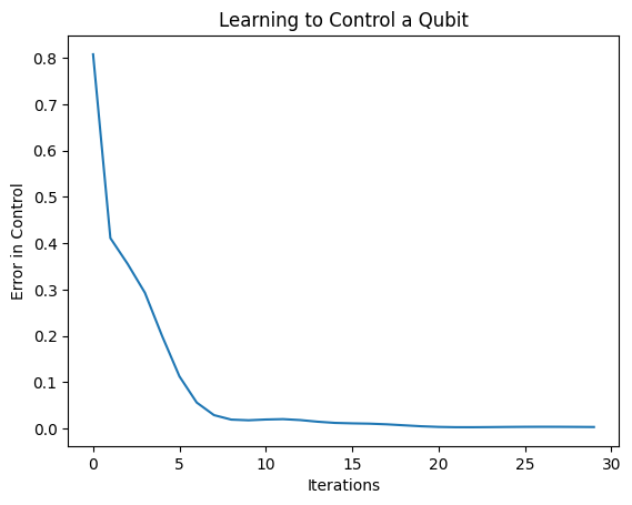
इस कथानक से आप देख सकते हैं कि तंत्रिका नेटवर्क ने व्यवस्थित गलत अंशांकन को दूर करना सीख लिया है।
2.6 आउटपुट सत्यापित करें
अब क्वेट कैलिब्रेशन त्रुटियों को ठीक करने के लिए प्रशिक्षित मॉडल का उपयोग करें। सर्क के साथ:
def check_error(command_values, desired_values):
  """Based on the value in `command_value` see how well you could prepare
  the full circuit to have `desired_value` when taking expectation w.r.t. Z."""
  params_to_prepare_output = controller(command_values).numpy()
  full_circuit = noisy_preparation + model_circuit

  # Test how well you can prepare a state to get expectation the expectation
  # value in `desired_values`
  for index in [0, 1]:
    state = cirq_simulator.simulate(
        full_circuit,
        {s:v for (s,v) in zip(control_params, params_to_prepare_output[index])}
    ).final_state_vector
    expt = cirq.Z(qubit).expectation_from_state_vector(state, {qubit: 0}).real
    print(f'For a desired output (expectation) of {desired_values[index]} with'
          f' noisy preparation, the controller\nnetwork found the following '
          f'values for theta: {params_to_prepare_output[index]}\nWhich gives an'
          f' actual expectation of: {expt}\n')


check_error(commands, expected_outputs)
For a desired output (expectation) of [1.] with noisy preparation, the controller
network found the following values for theta: [-0.6788422   0.3395225  -0.59394693]
Which gives an actual expectation of: 0.9171845316886902

For a desired output (expectation) of [-1.] with noisy preparation, the controller
network found the following values for theta: [-5.203663   -0.29528576  3.2887425 ]
Which gives an actual expectation of: -0.9511058330535889
प्रशिक्षण के दौरान नुकसान फ़ंक्शन का मूल्य यह अनुमान लगाता है कि मॉडल कितनी अच्छी तरह सीख रहा है। नुकसान जितना कम होगा, उपरोक्त सेल में अपेक्षित मान desired_values के करीब होंगे। यदि आप पैरामीटर मानों से उतने चिंतित नहीं हैं, तो आप हमेशा tfq का उपयोग करके ऊपर से आउटपुट की जांच कर सकते हैं:
model([datapoint_circuits, commands])
<tf.Tensor: shape=(2, 1), dtype=float32, numpy=
array([[ 0.91718477],
       [-0.9511056 ]], dtype=float32)>
3 विभिन्न ऑपरेटरों के स्वदेशी तैयार करना सीखना
1 और 0 के अनुरूप \(\pm \hat{Z}\) eigenstates का चुनाव मनमाना था। आप आसानी से 1 को \(+ \hat{Z}\) eigenstate के अनुरूप बनाना चाहते थे और 0 को \(-\hat{X}\) eigenstate के अनुरूप बनाना चाहते थे। इसे पूरा करने का एक तरीका प्रत्येक कमांड के लिए एक अलग माप ऑपरेटर निर्दिष्ट करना है, जैसा कि नीचे दिए गए चित्र में दर्शाया गया है:

इसके लिए tfq.layers.Expectation के उपयोग की आवश्यकता है। अब आपके इनपुट में तीन ऑब्जेक्ट शामिल हो गए हैं: सर्किट, कमांड और ऑपरेटर। आउटपुट अभी भी अपेक्षित मूल्य है।
3.1 नई मॉडल परिभाषा
आइए इस कार्य को पूरा करने के लिए मॉडल पर एक नज़र डालें:
# Define inputs.
commands_input = tf.keras.layers.Input(shape=(1),
                                       dtype=tf.dtypes.float32,
                                       name='commands_input')
circuits_input = tf.keras.Input(shape=(),
                                # The circuit-tensor has dtype `tf.string`
                                dtype=tf.dtypes.string,
                                name='circuits_input')
operators_input = tf.keras.Input(shape=(1,),
                                 dtype=tf.dtypes.string,
                                 name='operators_input')
यहाँ नियंत्रक नेटवर्क है:
# Define classical NN.
controller = tf.keras.Sequential([
    tf.keras.layers.Dense(10, activation='elu'),
    tf.keras.layers.Dense(3)
])
सर्किट और नियंत्रक को एक ही केरस में मिलाएं। keras.Model का उपयोग कर tfq :
dense_2 = controller(commands_input)

# Since you aren't using a PQC or ControlledPQC you must append
# your model circuit onto the datapoint circuit tensor manually.
full_circuit = tfq.layers.AddCircuit()(circuits_input, append=model_circuit)
expectation_output = tfq.layers.Expectation()(full_circuit,
                                              symbol_names=control_params,
                                              symbol_values=dense_2,
                                              operators=operators_input)

# Contruct your Keras model.
two_axis_control_model = tf.keras.Model(
    inputs=[circuits_input, commands_input, operators_input],
    outputs=[expectation_output])
3.2 डेटासेट
अब आप उन ऑपरेटरों को भी शामिल करेंगे जिन्हें आप प्रत्येक डेटापॉइंट के लिए मापना चाहते हैं जिसे आप model_circuit के लिए आपूर्ति करते हैं:
# The operators to measure, for each command.
operator_data = tfq.convert_to_tensor([[cirq.X(qubit)], [cirq.Z(qubit)]])

# The command input values to the classical NN.
commands = np.array([[0], [1]], dtype=np.float32)

# The desired expectation value at output of quantum circuit.
expected_outputs = np.array([[1], [-1]], dtype=np.float32)
3.3 प्रशिक्षण
अब जब आपके पास अपने नए इनपुट और आउटपुट हैं, तो आप केरस का उपयोग करके एक बार फिर से प्रशिक्षण ले सकते हैं।
optimizer = tf.keras.optimizers.Adam(learning_rate=0.05)
loss = tf.keras.losses.MeanSquaredError()

two_axis_control_model.compile(optimizer=optimizer, loss=loss)

history = two_axis_control_model.fit(
    x=[datapoint_circuits, commands, operator_data],
    y=expected_outputs,
    epochs=30,
    verbose=1)
Epoch 1/30
1/1 [==============================] - 0s 320ms/step - loss: 2.4404
Epoch 2/30
1/1 [==============================] - 0s 3ms/step - loss: 1.8713
Epoch 3/30
1/1 [==============================] - 0s 3ms/step - loss: 1.1400
Epoch 4/30
1/1 [==============================] - 0s 3ms/step - loss: 0.5071
Epoch 5/30
1/1 [==============================] - 0s 3ms/step - loss: 0.1611
Epoch 6/30
1/1 [==============================] - 0s 3ms/step - loss: 0.0426
Epoch 7/30
1/1 [==============================] - 0s 3ms/step - loss: 0.0117
Epoch 8/30
1/1 [==============================] - 0s 3ms/step - loss: 0.0032
Epoch 9/30
1/1 [==============================] - 0s 2ms/step - loss: 0.0147
Epoch 10/30
1/1 [==============================] - 0s 3ms/step - loss: 0.0452
Epoch 11/30
1/1 [==============================] - 0s 3ms/step - loss: 0.0670
Epoch 12/30
1/1 [==============================] - 0s 3ms/step - loss: 0.0648
Epoch 13/30
1/1 [==============================] - 0s 3ms/step - loss: 0.0471
Epoch 14/30
1/1 [==============================] - 0s 3ms/step - loss: 0.0289
Epoch 15/30
1/1 [==============================] - 0s 3ms/step - loss: 0.0180
Epoch 16/30
1/1 [==============================] - 0s 3ms/step - loss: 0.0138
Epoch 17/30
1/1 [==============================] - 0s 2ms/step - loss: 0.0130
Epoch 18/30
1/1 [==============================] - 0s 3ms/step - loss: 0.0137
Epoch 19/30
1/1 [==============================] - 0s 3ms/step - loss: 0.0148
Epoch 20/30
1/1 [==============================] - 0s 3ms/step - loss: 0.0156
Epoch 21/30
1/1 [==============================] - 0s 3ms/step - loss: 0.0157
Epoch 22/30
1/1 [==============================] - 0s 3ms/step - loss: 0.0149
Epoch 23/30
1/1 [==============================] - 0s 3ms/step - loss: 0.0135
Epoch 24/30
1/1 [==============================] - 0s 3ms/step - loss: 0.0119
Epoch 25/30
1/1 [==============================] - 0s 3ms/step - loss: 0.0100
Epoch 26/30
1/1 [==============================] - 0s 3ms/step - loss: 0.0082
Epoch 27/30
1/1 [==============================] - 0s 3ms/step - loss: 0.0064
Epoch 28/30
1/1 [==============================] - 0s 3ms/step - loss: 0.0047
Epoch 29/30
1/1 [==============================] - 0s 3ms/step - loss: 0.0034
Epoch 30/30
1/1 [==============================] - 0s 3ms/step - loss: 0.0024
plt.plot(history.history['loss'])
plt.title("Learning to Control a Qubit")
plt.xlabel("Iterations")
plt.ylabel("Error in Control")
plt.show()
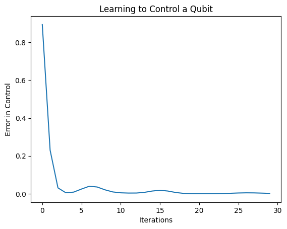
हानि समारोह शून्य हो गया है।
controller एक स्टैंड-अलोन मॉडल के रूप में उपलब्ध है। नियंत्रक को कॉल करें, और प्रत्येक कमांड सिग्नल पर उसकी प्रतिक्रिया जांचें। इन आउटपुट को random_rotations की सामग्री से सही ढंग से तुलना करने में कुछ काम लगेगा।
controller.predict(np.array([0,1]))
array([[3.6335812 , 1.8470774 , 0.71675825],
       [5.3085413 , 0.08116499, 2.8337662 ]], dtype=float32)