
| |  GitHubでソースを表示 GitHubでソースを表示 | |
行われた比較のオフ構築MNISTのチュートリアル、このチュートリアル探究の最近の作品Huangら。これは、さまざまなデータセットがパフォーマンスの比較にどのように影響するかを示しています。この研究では、著者は、古典的な機械学習モデルが量子モデルと同様に(またはそれよりも優れて)学習できる方法と時期を理解しようとしています。この作品はまた、慎重に作成されたデータセットを介して、古典的な機械学習モデルと量子機械学習モデルの間の経験的なパフォーマンスの分離を示しています。あなたはするであろう:
- 縮小された次元のFashion-MNISTデータセットを準備します。
- 量子回路を使用してデータセットにラベルを付け直し、Projected Quantum Kernel features(PQK)を計算します。
- 再ラベル付けされたデータセットで古典的なニューラルネットワークをトレーニングし、PQK機能にアクセスできるモデルとパフォーマンスを比較します。
設定
pip install tensorflow==2.4.1 tensorflow-quantum
# Update package resources to account for version changes.
import importlib, pkg_resources
importlib.reload(pkg_resources)
import cirq
import sympy
import numpy as np
import tensorflow as tf
import tensorflow_quantum as tfq

# visualization tools
%matplotlib inline
import matplotlib.pyplot as plt
from cirq.contrib.svg import SVGCircuit
np.random.seed(1234)
1.データの準備
まず、量子コンピューターで実行するためのファッションMNISTデータセットを準備します。
1.1ダウンロードファッション-MNIST
最初のステップは、従来のファッションミストデータセットを取得することです。これは、使用して行うことができるtf.keras.datasetsモジュールを。
(x_train, y_train), (x_test, y_test) = tf.keras.datasets.fashion_mnist.load_data()

# Rescale the images from [0,255] to the [0.0,1.0] range.
x_train, x_test = x_train/255.0, x_test/255.0

print("Number of original training examples:", len(x_train))
print("Number of original test examples:", len(x_test))
Number of original training examples: 60000
Number of original test examples: 10000
データセットをフィルタリングして、Tシャツ/トップスとドレスだけを保持し、他のクラスを削除します。同時にコンバートラベルでは、 y 、ブール値:0のためのTrueとFalse 3のために。
def filter_03(x, y):
    keep = (y == 0) | (y == 3)
    x, y = x[keep], y[keep]
    y = y == 0
    return x,y
x_train, y_train = filter_03(x_train, y_train)
x_test, y_test = filter_03(x_test, y_test)

print("Number of filtered training examples:", len(x_train))
print("Number of filtered test examples:", len(x_test))
Number of filtered training examples: 12000
Number of filtered test examples: 2000
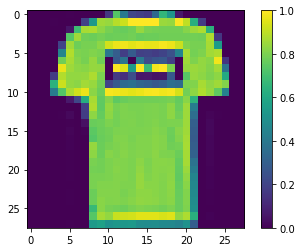
print(y_train[0])

plt.imshow(x_train[0, :, :])
plt.colorbar()
True
<matplotlib.colorbar.Colorbar at 0x7f6db42c3460>
1.2画像を縮小する
MNISTの例と同様に、現在の量子コンピューターの境界内に収まるようにするには、これらの画像をダウンスケールする必要があります。あなたが代わりの寸法減らすためにPCA変換を使用しますが、この時間tf.image.resize操作を。
def truncate_x(x_train, x_test, n_components=10):
  """Perform PCA on image dataset keeping the top `n_components` components."""
  n_points_train = tf.gather(tf.shape(x_train), 0)
  n_points_test = tf.gather(tf.shape(x_test), 0)

  # Flatten to 1D
  x_train = tf.reshape(x_train, [n_points_train, -1])
  x_test = tf.reshape(x_test, [n_points_test, -1])

  # Normalize.
  feature_mean = tf.reduce_mean(x_train, axis=0)
  x_train_normalized = x_train - feature_mean
  x_test_normalized = x_test - feature_mean

  # Truncate.
  e_values, e_vectors = tf.linalg.eigh(
      tf.einsum('ji,jk->ik', x_train_normalized, x_train_normalized))
  return tf.einsum('ij,jk->ik', x_train_normalized, e_vectors[:,-n_components:]), \
    tf.einsum('ij,jk->ik', x_test_normalized, e_vectors[:, -n_components:])
DATASET_DIM = 10
x_train, x_test = truncate_x(x_train, x_test, n_components=DATASET_DIM)
print(f'New datapoint dimension:', len(x_train[0]))
New datapoint dimension: 10
最後のステップは、データセットのサイズを1000個のトレーニングデータポイントと200個のテストデータポイントに減らすことです。
N_TRAIN = 1000
N_TEST = 200
x_train, x_test = x_train[:N_TRAIN], x_test[:N_TEST]
y_train, y_test = y_train[:N_TRAIN], y_test[:N_TEST]
print("New number of training examples:", len(x_train))
print("New number of test examples:", len(x_test))
New number of training examples: 1000
New number of test examples: 200
2.PQK機能のラベル変更と計算
ここで、量子コンポーネントを組み込み、上記で作成した切り捨てられたファッションMNISTデータセットにラベルを付け直すことにより、「高床式」量子データセットを準備します。クォンタムメソッドとクラシックメソッドを最大限に分離するために、最初にPQK機能を準備し、次にそれらの値に基づいて出力にラベルを付け直します。
2.1量子エンコーディングとPQK機能
あなたがに基づいて、機能の新しいセットを作成しますx_train 、 y_train 、 x_testとy_testのすべての量子ビットの1-RDMになるように定義されています。
\(V(x_{\text{train} } / n_{\text{trotter} }) ^ {n_{\text{trotter} } } U_{\text{1qb} } | 0 \rangle\)
どこ \(U_\text{1qb}\) 、単一の量子ビットの回転との壁である \(V(\hat{\theta}) = e^{-i\sum_i \hat{\theta_i} (X_i X_{i+1} + Y_i Y_{i+1} + Z_i Z_{i+1})}\)
まず、単一キュービット回転の壁を生成できます。
def single_qubit_wall(qubits, rotations):
  """Prepare a single qubit X,Y,Z rotation wall on `qubits`."""
  wall_circuit = cirq.Circuit()
  for i, qubit in enumerate(qubits):
    for j, gate in enumerate([cirq.X, cirq.Y, cirq.Z]):
      wall_circuit.append(gate(qubit) ** rotations[i][j])

  return wall_circuit
回路を調べることで、これが機能することをすばやく確認できます。
SVGCircuit(single_qubit_wall(
    cirq.GridQubit.rect(1,4), np.random.uniform(size=(4, 3))))

あなたが準備することができます次 \(V(\hat{\theta})\) の助けを借りてtfq.util.exponential任意の通勤累乗することができますcirq.PauliSumオブジェクト:
def v_theta(qubits):
  """Prepares a circuit that generates V(\theta)."""
  ref_paulis = [
      cirq.X(q0) * cirq.X(q1) + \
      cirq.Y(q0) * cirq.Y(q1) + \
      cirq.Z(q0) * cirq.Z(q1) for q0, q1 in zip(qubits, qubits[1:])
  ]
  exp_symbols = list(sympy.symbols('ref_0:'+str(len(ref_paulis))))
  return tfq.util.exponential(ref_paulis, exp_symbols), exp_symbols
この回路を見て確認するのは少し難しいかもしれませんが、それでも2キュービットのケースを調べて何が起こっているかを確認できます。
test_circuit, test_symbols = v_theta(cirq.GridQubit.rect(1, 2))
print(f'Symbols found in circuit:{test_symbols}')
SVGCircuit(test_circuit)
Symbols found in circuit:[ref_0]

これで、完全なエンコーディング回路をまとめるのに必要なすべてのビルディングブロックができました。
def prepare_pqk_circuits(qubits, classical_source, n_trotter=10):
  """Prepare the pqk feature circuits around a dataset."""
  n_qubits = len(qubits)
  n_points = len(classical_source)

  # Prepare random single qubit rotation wall.
  random_rots = np.random.uniform(-2, 2, size=(n_qubits, 3))
  initial_U = single_qubit_wall(qubits, random_rots)

  # Prepare parametrized V
  V_circuit, symbols = v_theta(qubits)
  exp_circuit = cirq.Circuit(V_circuit for t in range(n_trotter))

  # Convert to `tf.Tensor`
  initial_U_tensor = tfq.convert_to_tensor([initial_U])
  initial_U_splat = tf.tile(initial_U_tensor, [n_points])

  full_circuits = tfq.layers.AddCircuit()(
      initial_U_splat, append=exp_circuit)
  # Replace placeholders in circuits with values from `classical_source`.
  return tfq.resolve_parameters(
      full_circuits, tf.convert_to_tensor([str(x) for x in symbols]),
      tf.convert_to_tensor(classical_source*(n_qubits/3)/n_trotter))
いくつかの量子ビットを選択し、データエンコーディング回路を準備します。
qubits = cirq.GridQubit.rect(1, DATASET_DIM + 1)
q_x_train_circuits = prepare_pqk_circuits(qubits, x_train)
q_x_test_circuits = prepare_pqk_circuits(qubits, x_test)
次に、PQKデータセット回路上とで結果格納の1-RDMに基づいて特徴を計算rdm 、 tf.Tensor形状の[n_points, n_qubits, 3]エントリrdm[i][j][k] = \(\langle \psi_i | OP^k_j | \psi_i \rangle\) iインデックスデータポイント、上j量子ビットとに対する索引kに対する索引 \(\lbrace \hat{X}, \hat{Y}, \hat{Z} \rbrace\) 。
def get_pqk_features(qubits, data_batch):
  """Get PQK features based on above construction."""
  ops = [[cirq.X(q), cirq.Y(q), cirq.Z(q)] for q in qubits]
  ops_tensor = tf.expand_dims(tf.reshape(tfq.convert_to_tensor(ops), -1), 0)
  batch_dim = tf.gather(tf.shape(data_batch), 0)
  ops_splat = tf.tile(ops_tensor, [batch_dim, 1])
  exp_vals = tfq.layers.Expectation()(data_batch, operators=ops_splat)
  rdm = tf.reshape(exp_vals, [batch_dim, len(qubits), -1])
  return rdm
x_train_pqk = get_pqk_features(qubits, q_x_train_circuits)
x_test_pqk = get_pqk_features(qubits, q_x_test_circuits)
print('New PQK training dataset has shape:', x_train_pqk.shape)
print('New PQK testing dataset has shape:', x_test_pqk.shape)
New PQK training dataset has shape: (1000, 11, 3)
New PQK testing dataset has shape: (200, 11, 3)
2.2PQK機能に基づく再ラベル付け
今、あなたは、これらの量子生成の機能を持っていることをx_train_pqkとx_test_pqk 、それが再ラベルデータセットまでの時間です。量子と古典パフォーマンスとの間の最大の別離を達成するためにあなたが再ラベルを付けることができスペクトル情報に基づいてデータセットがで見つかったx_train_pqkとx_test_pqk 。
def compute_kernel_matrix(vecs, gamma):
  """Computes d[i][j] = e^ -gamma * (vecs[i] - vecs[j]) ** 2 """
  scaled_gamma = gamma / (
      tf.cast(tf.gather(tf.shape(vecs), 1), tf.float32) * tf.math.reduce_std(vecs))
  return scaled_gamma * tf.einsum('ijk->ij',(vecs[:,None,:] - vecs) ** 2)

def get_spectrum(datapoints, gamma=1.0):
  """Compute the eigenvalues and eigenvectors of the kernel of datapoints."""
  KC_qs = compute_kernel_matrix(datapoints, gamma)
  S, V = tf.linalg.eigh(KC_qs)
  S = tf.math.abs(S)
  return S, V
S_pqk, V_pqk = get_spectrum(
    tf.reshape(tf.concat([x_train_pqk, x_test_pqk], 0), [-1, len(qubits) * 3]))

S_original, V_original = get_spectrum(
    tf.cast(tf.concat([x_train, x_test], 0), tf.float32), gamma=0.005)

print('Eigenvectors of pqk kernel matrix:', V_pqk)
print('Eigenvectors of original kernel matrix:', V_original)
Eigenvectors of pqk kernel matrix: tf.Tensor(
[[-2.09569391e-02  1.05973557e-02  2.16634180e-02 ...  2.80352887e-02
   1.55521873e-02  2.82677952e-02]
 [-2.29303762e-02  4.66355234e-02  7.91163836e-03 ... -6.14174758e-04
  -7.07804322e-01  2.85902526e-02]
 [-1.77853629e-02 -3.00758495e-03 -2.55225878e-02 ... -2.40783971e-02
   2.11018627e-03  2.69009806e-02]
 ...
 [ 6.05797209e-02  1.32483775e-02  2.69536003e-02 ... -1.38843581e-02
   3.05043962e-02  3.85345481e-02]
 [ 6.33309558e-02 -3.04112374e-03  9.77444276e-03 ...  7.48321265e-02
   3.42793856e-03  3.67484428e-02]
 [ 5.86028099e-02  5.84433973e-03  2.64811981e-03 ...  2.82612257e-02
  -3.80136147e-02  3.29943895e-02]], shape=(1200, 1200), dtype=float32)
Eigenvectors of original kernel matrix: tf.Tensor(
[[ 0.03835681  0.0283473  -0.01169789 ...  0.02343717  0.0211248
   0.03206972]
 [-0.04018159  0.00888097 -0.01388255 ...  0.00582427  0.717551
   0.02881948]
 [-0.0166719   0.01350376 -0.03663862 ...  0.02467175 -0.00415936
   0.02195409]
 ...
 [-0.03015648 -0.01671632 -0.01603392 ...  0.00100583 -0.00261221
   0.02365689]
 [ 0.0039777  -0.04998879 -0.00528336 ...  0.01560401 -0.04330755
   0.02782002]
 [-0.01665728 -0.00818616 -0.0432341  ...  0.00088256  0.00927396
   0.01875088]], shape=(1200, 1200), dtype=float32)
これで、データセットのラベルを変更するために必要なものがすべて揃いました。これで、フローチャートを参照して、データセットにラベルを付け直すときにパフォーマンスの分離を最大化する方法をよりよく理解できます。
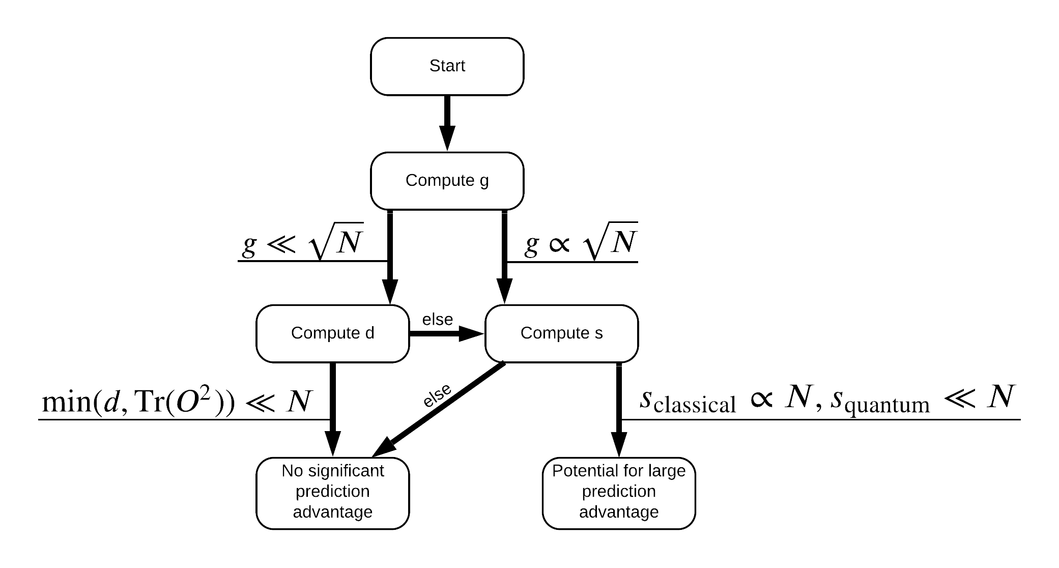
量子と古典モデル間の別離を最大化するために、あなたは、元のデータセット間の幾何学的な差異を最大化しようとするとPQKは、カーネル行列ます \(g(K_1 || K_2) = \sqrt{ || \sqrt{K_2} K_1^{-1} \sqrt{K_2} || _\infty}\) 使用S_pqk, V_pqkとS_original, V_original 。大きな値 \(g\) 最初に量子場合の予測利点に向けたフローチャートの下に右に移動することを保証します。
def get_stilted_dataset(S, V, S_2, V_2, lambdav=1.1):
  """Prepare new labels that maximize geometric distance between kernels."""
  S_diag = tf.linalg.diag(S ** 0.5)
  S_2_diag = tf.linalg.diag(S_2 / (S_2 + lambdav) ** 2)
  scaling = S_diag @ tf.transpose(V) @ \
            V_2 @ S_2_diag @ tf.transpose(V_2) @ \
            V @ S_diag

  # Generate new lables using the largest eigenvector.
  _, vecs = tf.linalg.eig(scaling)
  new_labels = tf.math.real(
      tf.einsum('ij,j->i', tf.cast(V @ S_diag, tf.complex64), vecs[-1])).numpy()
  # Create new labels and add some small amount of noise.
  final_y = new_labels > np.median(new_labels)
  noisy_y = (final_y ^ (np.random.uniform(size=final_y.shape) > 0.95))
  return noisy_y
y_relabel = get_stilted_dataset(S_pqk, V_pqk, S_original, V_original)
y_train_new, y_test_new = y_relabel[:N_TRAIN], y_relabel[N_TRAIN:]
3.モデルの比較
データセットを準備したので、モデルのパフォーマンスを比較します。あなたは二つの小さなフィードフォワードニューラルネットワークを作成し、それらが中に見られる特徴PQKへのアクセス権を与えられたときのパフォーマンスを比較しますx_train_pqk 。
3.1PQK拡張モデルを作成する
標準使用tf.kerasあなたが今でモデルを作成し、訓練することができ、ライブラリの機能x_train_pqkとy_train_newデータポイントを:
#docs_infra: no_execute
def create_pqk_model():
    model = tf.keras.Sequential()
    model.add(tf.keras.layers.Dense(32, activation='sigmoid', input_shape=[len(qubits) * 3,]))
    model.add(tf.keras.layers.Dense(16, activation='sigmoid'))
    model.add(tf.keras.layers.Dense(1))
    return model

pqk_model = create_pqk_model()
pqk_model.compile(loss=tf.keras.losses.BinaryCrossentropy(from_logits=True),
              optimizer=tf.keras.optimizers.Adam(learning_rate=0.003),
              metrics=['accuracy'])

pqk_model.summary()
Model: "sequential"
_________________________________________________________________
Layer (type)                 Output Shape              Param #
=================================================================
dense (Dense)                (None, 32)                1088
_________________________________________________________________
dense_1 (Dense)              (None, 16)                528
_________________________________________________________________
dense_2 (Dense)              (None, 1)                 17
=================================================================
Total params: 1,633
Trainable params: 1,633
Non-trainable params: 0
_________________________________________________________________
#docs_infra: no_execute
pqk_history = pqk_model.fit(tf.reshape(x_train_pqk, [N_TRAIN, -1]),
          y_train_new,
          batch_size=32,
          epochs=1000,
          verbose=0,
          validation_data=(tf.reshape(x_test_pqk, [N_TEST, -1]), y_test_new))
3.2古典的なモデルを作成する
上記のコードと同様に、高床式データセットのPQK機能にアクセスできない従来のモデルを作成することもできます。このモデルは、使用してトレーニングすることができるx_trainとy_label_new 。
#docs_infra: no_execute
def create_fair_classical_model():
    model = tf.keras.Sequential()
    model.add(tf.keras.layers.Dense(32, activation='sigmoid', input_shape=[DATASET_DIM,]))
    model.add(tf.keras.layers.Dense(16, activation='sigmoid'))
    model.add(tf.keras.layers.Dense(1))
    return model

model = create_fair_classical_model()
model.compile(loss=tf.keras.losses.BinaryCrossentropy(from_logits=True),
              optimizer=tf.keras.optimizers.Adam(learning_rate=0.03),
              metrics=['accuracy'])

model.summary()
Model: "sequential_1"
_________________________________________________________________
Layer (type)                 Output Shape              Param #
=================================================================
dense_3 (Dense)              (None, 32)                352
_________________________________________________________________
dense_4 (Dense)              (None, 16)                528
_________________________________________________________________
dense_5 (Dense)              (None, 1)                 17
=================================================================
Total params: 897
Trainable params: 897
Non-trainable params: 0
_________________________________________________________________
#docs_infra: no_execute
classical_history = model.fit(x_train,
          y_train_new,
          batch_size=32,
          epochs=1000,
          verbose=0,
          validation_data=(x_test, y_test_new))
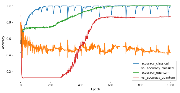
3.3パフォーマンスの比較
2つのモデルをトレーニングしたので、2つの間の検証データのパフォーマンスギャップをすばやくプロットできます。通常、両方のモデルは、トレーニングデータで0.9を超える精度を達成します。ただし、検証データでは、PQK機能で見つかった情報だけで、モデルを目に見えないインスタンスに適切に一般化するのに十分であることが明らかになります。
#docs_infra: no_execute
plt.figure(figsize=(10,5))
plt.plot(classical_history.history['accuracy'], label='accuracy_classical')
plt.plot(classical_history.history['val_accuracy'], label='val_accuracy_classical')
plt.plot(pqk_history.history['accuracy'], label='accuracy_quantum')
plt.plot(pqk_history.history['val_accuracy'], label='val_accuracy_quantum')
plt.xlabel('Epoch')
plt.ylabel('Accuracy')
plt.legend()
<matplotlib.legend.Legend at 0x7f6d846ecee0>
4.重要な結論
あなたはこのから引き出すことができ、いくつかの重要な結論がありますMNISTの実験は:
今日の量子モデルが古典的なデータの古典的なモデルのパフォーマンスを上回る可能性はほとんどありません。特に、100万を超えるデータポイントを持つ可能性のある今日の古典的なデータセットでは。
データが古典的に量子回路をシミュレートするのが難しいから来ているかもしれないという理由だけで、必ずしも古典的なモデルのためにデータを学ぶのを難しくするわけではありません。
使用するモデルアーキテクチャやトレーニングアルゴリズムに関係なく、量子モデルが学習しやすく、古典的なモデルが学習しにくいデータセット(最終的には量子)が存在します。