
| |  GitHubでソースを表示 GitHubでソースを表示 | |
このチュートリアルには、単語の埋め込みの概要が含まれています。感情分類タスク用の単純なKerasモデルを使用して独自の単語埋め込みをトレーニングし、埋め込みプロジェクター(下の画像に表示)でそれらを視覚化します。

テキストを数字で表す
機械学習モデルは、入力としてベクトル(数値の配列)を取ります。テキストを操作する場合、最初に行う必要があるのは、モデルにフィードする前に、文字列を数値に変換する(またはテキストを「ベクトル化」する)戦略を考え出すことです。このセクションでは、そうするための3つの戦略を見ていきます。
ワンホットエンコーディング
最初のアイデアとして、語彙の各単語を「ワンホット」でエンコードすることができます。 「猫がマットの上に座った」という文を考えてみましょう。この文の語彙(またはユニークな単語)は(cat、mat、on、sat、the)です。各単語を表すには、語彙に等しい長さのゼロベクトルを作成し、その単語に対応するインデックスに1を配置します。このアプローチを次の図に示します。
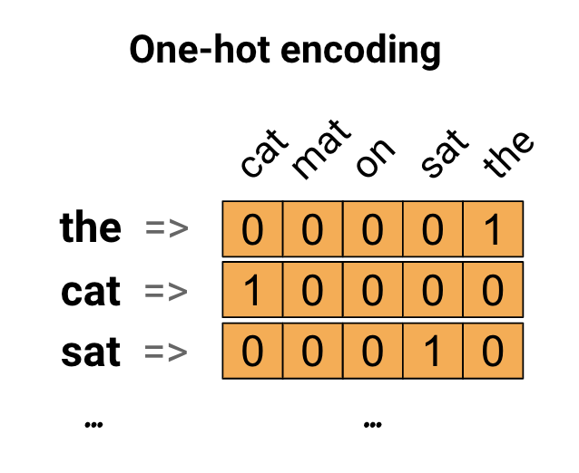
文のエンコーディングを含むベクトルを作成するには、各単語のワンホットベクトルを連結します。
各単語を一意の番号でエンコードします
あなたが試みるかもしれない2番目のアプローチは、一意の番号を使用して各単語をエンコードすることです。上記の例を続けると、1を「猫」に、2を「マット」に割り当てることができます。次に、「猫はマットの上に座った」という文を[5、1、4、3、5、2]のような密なベクトルとしてエンコードできます。このアプローチは効率的です。スパースベクトルの代わりに、密度の高いベクトルが作成されました(すべての要素がいっぱいになります)。
ただし、このアプローチには2つの欠点があります。
整数エンコードは任意です(単語間の関係はキャプチャされません)。
整数エンコーディングは、モデルが解釈するのが難しい場合があります。たとえば、線形分類器は、特徴ごとに1つの重みを学習します。 2つの単語の類似性とそれらのエンコーディングの類似性の間には関係がないため、この特徴と重みの組み合わせは意味がありません。
単語の埋め込み
単語の埋め込みは、類似した単語が類似したエンコーディングを持つ効率的で密な表現を使用する方法を提供します。重要なのは、このエンコーディングを手動で指定する必要がないことです。埋め込みは、浮動小数点値の密なベクトルです(ベクトルの長さは指定したパラメーターです)。埋め込みの値を手動で指定する代わりに、それらはトレーニング可能なパラメーターです(モデルが密なレイヤーの重みを学習するのと同じ方法で、トレーニング中にモデルによって学習された重み)。大きなデータセットを操作する場合、8次元(小さなデータセットの場合)、最大1024次元の単語の埋め込みがよく見られます。高次元の埋め込みは、単語間のきめ細かい関係をキャプチャできますが、学習するにはより多くのデータが必要です。
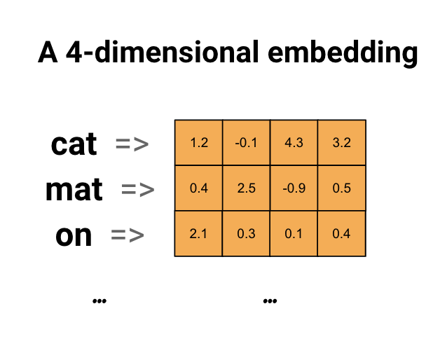
上の図は単語の埋め込みの図です。各単語は、浮動小数点値の4次元ベクトルとして表されます。埋め込みを考える別の方法は、「ルックアップテーブル」です。これらの重みが学習された後、テーブルで対応する密なベクトルを検索することにより、各単語をエンコードできます。
設定
import io
import os
import re
import shutil
import string
import tensorflow as tf

from tensorflow.keras import Sequential
from tensorflow.keras.layers import Dense, Embedding, GlobalAveragePooling1D
from tensorflow.keras.layers import TextVectorization
IMDbデータセットをダウンロードする
チュートリアルでは、ラージムービーレビューデータセットを使用します。このデータセットで感情分類モデルをトレーニングし、その過程で埋め込みを最初から学習します。データセットを最初から読み込む方法の詳細については、テキストの読み込みチュートリアルをご覧ください。
Kerasファイルユーティリティを使用してデータセットをダウンロードし、ディレクトリを確認します。
url = "https://ai.stanford.edu/~amaas/data/sentiment/aclImdb_v1.tar.gz"

dataset = tf.keras.utils.get_file("aclImdb_v1.tar.gz", url,
                                  untar=True, cache_dir='.',
                                  cache_subdir='')

dataset_dir = os.path.join(os.path.dirname(dataset), 'aclImdb')
os.listdir(dataset_dir)
Downloading data from https://ai.stanford.edu/~amaas/data/sentiment/aclImdb_v1.tar.gz
84131840/84125825 [==============================] - 7s 0us/step
84140032/84125825 [==============================] - 7s 0us/step
['test', 'imdb.vocab', 'imdbEr.txt', 'train', 'README']
train/ディレクトリを見てください。 posフォルダーとnegフォルダーがあり、映画レビューにはそれぞれポジティブとネガティブのラベルが付いています。 posフォルダーとnegフォルダーからのレビューを使用して、バイナリ分類モデルをトレーニングします。
train_dir = os.path.join(dataset_dir, 'train')
os.listdir(train_dir)
['urls_pos.txt',
 'urls_unsup.txt',
 'urls_neg.txt',
 'pos',
 'unsup',
 'unsupBow.feat',
 'neg',
 'labeledBow.feat']
trainディレクトリには、トレーニングデータセットを作成する前に削除する必要がある追加のフォルダもあります。
remove_dir = os.path.join(train_dir, 'unsup')
shutil.rmtree(remove_dir)
次に、 tf.data.Dataset tf.keras.utils.text_dataset_from_directory作成します。このユーティリティの使用について詳しくは、このテキスト分類チュートリアルをご覧ください。
trainディレクトリを使用して、検証用に20%の分割でトレインデータセットと検証データセットの両方を作成します。
batch_size = 1024
seed = 123
train_ds = tf.keras.utils.text_dataset_from_directory(
    'aclImdb/train', batch_size=batch_size, validation_split=0.2,
    subset='training', seed=seed)
val_ds = tf.keras.utils.text_dataset_from_directory(
    'aclImdb/train', batch_size=batch_size, validation_split=0.2,
    subset='validation', seed=seed)
Found 25000 files belonging to 2 classes.
Using 20000 files for training.
Found 25000 files belonging to 2 classes.
Using 5000 files for validation.
電車のデータセットからいくつかの映画レビューとそのラベル(1: positive, 0: negative)を見てください。
for text_batch, label_batch in train_ds.take(1):
  for i in range(5):
    print(label_batch[i].numpy(), text_batch.numpy()[i])
0 b"Oh My God! Please, for the love of all that is holy, Do Not Watch This Movie! It it 82 minutes of my life I will never get back. Sure, I could have stopped watching half way through. But I thought it might get better. It Didn't. Anyone who actually enjoyed this movie is one seriously sick and twisted individual. No wonder us Australians/New Zealanders have a terrible reputation when it comes to making movies. Everything about this movie is horrible, from the acting to the editing. I don't even normally write reviews on here, but in this case I'll make an exception. I only wish someone had of warned me before I hired this catastrophe"
1 b'This movie is SOOOO funny!!! The acting is WONDERFUL, the Ramones are sexy, the jokes are subtle, and the plot is just what every high schooler dreams of doing to his/her school. I absolutely loved the soundtrack as well as the carefully placed cynicism. If you like monty python, You will love this film. This movie is a tad bit "grease"esk (without all the annoying songs). The songs that are sung are likable; you might even find yourself singing these songs once the movie is through. This musical ranks number two in musicals to me (second next to the blues brothers). But please, do not think of it as a musical per say; seeing as how the songs are so likable, it is hard to tell a carefully choreographed scene is taking place. I think of this movie as more of a comedy with undertones of romance. You will be reminded of what it was like to be a rebellious teenager; needless to say, you will be reminiscing of your old high school days after seeing this film. Highly recommended for both the family (since it is a very youthful but also for adults since there are many jokes that are funnier with age and experience.'
0 b"Alex D. Linz replaces Macaulay Culkin as the central figure in the third movie in the Home Alone empire. Four industrial spies acquire a missile guidance system computer chip and smuggle it through an airport inside a remote controlled toy car. Because of baggage confusion, grouchy Mrs. Hess (Marian Seldes) gets the car. She gives it to her neighbor, Alex (Linz), just before the spies turn up. The spies rent a house in order to burglarize each house in the neighborhood until they locate the car. Home alone with the chicken pox, Alex calls 911 each time he spots a theft in progress, but the spies always manage to elude the police while Alex is accused of making prank calls. The spies finally turn their attentions toward Alex, unaware that he has rigged devices to cleverly booby-trap his entire house. Home Alone 3 wasn't horrible, but probably shouldn't have been made, you can't just replace Macauley Culkin, Joe Pesci, or Daniel Stern. Home Alone 3 had some funny parts, but I don't like when characters are changed in a movie series, view at own risk."
0 b"There's a good movie lurking here, but this isn't it. The basic idea is good: to explore the moral issues that would face a group of young survivors of the apocalypse. But the logic is so muddled that it's impossible to get involved.<br /><br />For example, our four heroes are (understandably) paranoid about catching the mysterious airborne contagion that's wiped out virtually all of mankind. Yet they wear surgical masks some times, not others. Some times they're fanatical about wiping down with bleach any area touched by an infected person. Other times, they seem completely unconcerned.<br /><br />Worse, after apparently surviving some weeks or months in this new kill-or-be-killed world, these people constantly behave like total newbs. They don't bother accumulating proper equipment, or food. They're forever running out of fuel in the middle of nowhere. They don't take elementary precautions when meeting strangers. And after wading through the rotting corpses of the entire human race, they're as squeamish as sheltered debutantes. You have to constantly wonder how they could have survived this long... and even if they did, why anyone would want to make a movie about them.<br /><br />So when these dweebs stop to agonize over the moral dimensions of their actions, it's impossible to take their soul-searching seriously. Their actions would first have to make some kind of minimal sense.<br /><br />On top of all this, we must contend with the dubious acting abilities of Chris Pine. His portrayal of an arrogant young James T Kirk might have seemed shrewd, when viewed in isolation. But in Carriers he plays on exactly that same note: arrogant and boneheaded. It's impossible not to suspect that this constitutes his entire dramatic range.<br /><br />On the positive side, the film *looks* excellent. It's got an over-sharp, saturated look that really suits the southwestern US locale. But that can't save the truly feeble writing nor the paper-thin (and annoying) characters. Even if you're a fan of the end-of-the-world genre, you should save yourself the agony of watching Carriers."
0 b'I saw this movie at an actual movie theater (probably the \\(2.00 one) with my cousin and uncle. We were around 11 and 12, I guess, and really into scary movies. I remember being so excited to see it because my cool uncle let us pick the movie (and we probably never got to do that again!) and sooo disappointed afterwards!! Just boring and not scary. The only redeeming thing I can remember was Corky Pigeon from Silver Spoons, and that wasn\'t all that great, just someone I recognized. I\'ve seen bad movies before and this one has always stuck out in my mind as the worst. This was from what I can recall, one of the most boring, non-scary, waste of our collective \\)6, and a waste of film. I have read some of the reviews that say it is worth a watch and I say, "Too each his own", but I wouldn\'t even bother. Not even so bad it\'s good.'
パフォーマンスのためにデータセットを構成する
これらは、I / Oがブロックされないようにするためにデータをロードするときに使用する必要がある2つの重要な方法です。
.cache()は、データがディスクからロードされた後、データをメモリに保持します。これにより、モデルのトレーニング中にデータセットがボトルネックにならないようになります。データセットが大きすぎてメモリに収まらない場合は、この方法を使用して、パフォーマンスの高いオンディスクキャッシュを作成することもできます。これは、多くの小さなファイルよりも効率的に読み取ることができます。
.prefetch()は、トレーニング中のデータの前処理とモデルの実行をオーバーラップさせます。
データパフォーマンスガイドで、両方の方法と、データをディスクにキャッシュする方法について詳しく知ることができます。
AUTOTUNE = tf.data.AUTOTUNE

train_ds = train_ds.cache().prefetch(buffer_size=AUTOTUNE)
val_ds = val_ds.cache().prefetch(buffer_size=AUTOTUNE)
埋め込みレイヤーの使用
Kerasを使用すると、単語の埋め込みを簡単に使用できます。埋め込みレイヤーを見てください。
埋め込みレイヤーは、整数インデックス(特定の単語を表す)から高密度ベクトル(埋め込み)にマップするルックアップテーブルとして理解できます。埋め込みの次元(または幅)は、密な層のニューロンの数を実験するのとほぼ同じ方法で、問題に対して何がうまく機能するかを確認するために実験できるパラメーターです。
# Embed a 1,000 word vocabulary into 5 dimensions.
embedding_layer = tf.keras.layers.Embedding(1000, 5)
埋め込みレイヤーを作成すると、埋め込みの重みがランダムに初期化されます(他のレイヤーと同じように)。トレーニング中、バックプロパゲーションによって徐々に調整されます。トレーニングされると、学習された単語の埋め込みは、単語間の類似性を大まかにエンコードします(モデルがトレーニングされている特定の問題について学習されたため)。
整数を埋め込みレイヤーに渡すと、結果は各整数を埋め込みテーブルのベクトルに置き換えます。
result = embedding_layer(tf.constant([1, 2, 3]))
result.numpy()
array([[ 0.01318491, -0.02219239,  0.024673  , -0.03208025,  0.02297195],
       [-0.00726584,  0.03731754, -0.01209557, -0.03887399, -0.02407478],
       [ 0.04477594,  0.04504738, -0.02220147, -0.03642888, -0.04688282]],
      dtype=float32)
テキストまたはシーケンスの問題の場合、埋め込みレイヤーは、形状(samples, sequence_length)の整数の2Dテンソルを取ります。ここで、各エントリは整数のシーケンスです。可変長のシーケンスを埋め込むことができます。形状(32, 10) (長さ10の32シーケンスのバッチ)または(64, 15) (長さ15の64シーケンスのバッチ)のバッチの上の埋め込みレイヤーにフィードできます。
返されるテンソルには入力よりも1つ多い軸があり、埋め込みベクトルは新しい最後の軸に沿って整列されます。 (2, 3)入力バッチを渡すと、出力は(2, 3, N)なります。
result = embedding_layer(tf.constant([[0, 1, 2], [3, 4, 5]]))
result.shape
TensorShape([2, 3, 5])
シーケンスのバッチが入力として与えられると、埋め込みレイヤーは、形状(samples, sequence_length, embedding_dimensionality)の3D浮動小数点テンソルを返します。この可変長のシーケンスから固定表現に変換するには、さまざまな標準的なアプローチがあります。 Denseレイヤーに渡す前に、RNN、Attention、またはプーリングレイヤーを使用できます。このチュートリアルでは、最も単純なため、プーリングを使用します。 RNNチュートリアルを使用したテキスト分類は、次の良いステップです。
テキストの前処理
次に、感情分類モデルに必要なデータセットの前処理ステップを定義します。映画レビューをベクトル化するために、必要なパラメーターを使用してTextVectorizationレイヤーを初期化します。このレイヤーの使用について詳しくは、テキスト分類チュートリアルをご覧ください。
# Create a custom standardization function to strip HTML break tags '<br />'.
def custom_standardization(input_data):
  lowercase = tf.strings.lower(input_data)
  stripped_html = tf.strings.regex_replace(lowercase, '<br />', ' ')
  return tf.strings.regex_replace(stripped_html,
                                  '[%s]' % re.escape(string.punctuation), '')


# Vocabulary size and number of words in a sequence.
vocab_size = 10000
sequence_length = 100

# Use the text vectorization layer to normalize, split, and map strings to
# integers. Note that the layer uses the custom standardization defined above.
# Set maximum_sequence length as all samples are not of the same length.
vectorize_layer = TextVectorization(
    standardize=custom_standardization,
    max_tokens=vocab_size,
    output_mode='int',
    output_sequence_length=sequence_length)

# Make a text-only dataset (no labels) and call adapt to build the vocabulary.
text_ds = train_ds.map(lambda x, y: x)
vectorize_layer.adapt(text_ds)
分類モデルを作成する
Keras Sequential APIを使用して、感情分類モデルを定義します。この場合、それは「言葉の連続バッグ」スタイルのモデルです。
-
TextVectorizationレイヤーは、文字列を語彙インデックスに変換します。すでにvectorize_layerをTextVectorizationレイヤーとして初期化し、text_dsでadaptを呼び出してその語彙を構築しました。これで、vectorize_layerをエンドツーエンドの分類モデルの最初のレイヤーとして使用して、変換された文字列を埋め込みレイヤーにフィードできます。 Embeddingレイヤーは、整数でエンコードされた語彙を取得し、各単語インデックスの埋め込みベクトルを検索します。これらのベクトルは、鉄道模型として学習されます。ベクトルは、出力配列に次元を追加します。結果のディメンションは次のとおりです:((batch, sequence, embedding)。GlobalAveragePooling1Dレイヤーは、シーケンスディメンションを平均化することにより、各例の固定長の出力ベクトルを返します。これにより、モデルは可能な限り簡単な方法で可変長の入力を処理できます。固定長の出力ベクトルは、16個の非表示ユニットを持つ完全に接続された(
Dense)レイヤーを介してパイプされます。最後のレイヤーは、単一の出力ノードに密に接続されています。
embedding_dim=16

model = Sequential([
  vectorize_layer,
  Embedding(vocab_size, embedding_dim, name="embedding"),
  GlobalAveragePooling1D(),
  Dense(16, activation='relu'),
  Dense(1)
])
モデルをコンパイルしてトレーニングする
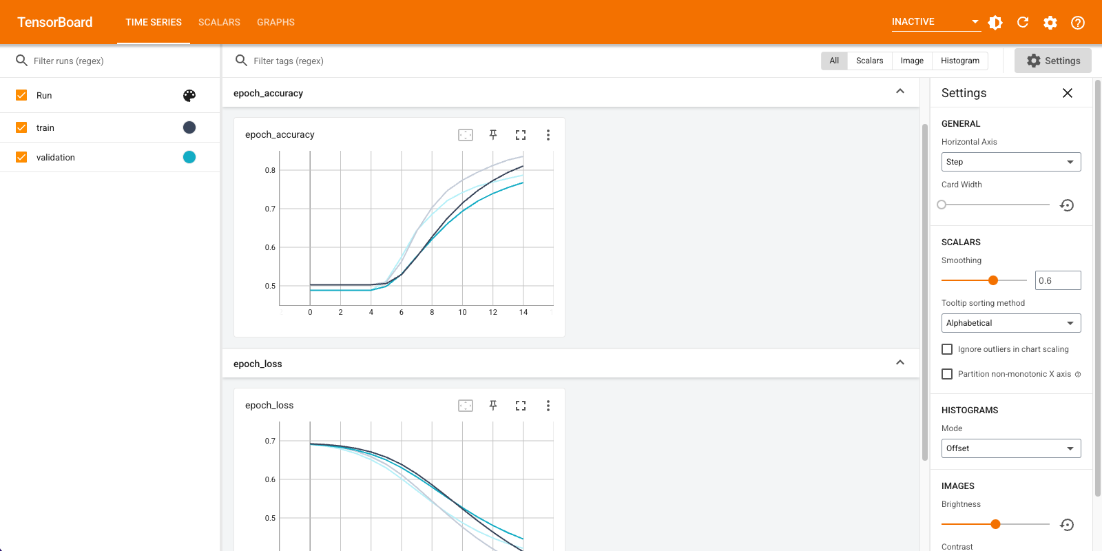
TensorBoardを使用して、損失や精度などの指標を視覚化します。 tf.keras.callbacks.TensorBoardを作成します。
tensorboard_callback = tf.keras.callbacks.TensorBoard(log_dir="logs")
AdamオプティマイザーとBinaryCrossentropy損失を使用して、モデルをコンパイルおよびトレーニングします。
model.compile(optimizer='adam',
              loss=tf.keras.losses.BinaryCrossentropy(from_logits=True),
              metrics=['accuracy'])
model.fit(
    train_ds,
    validation_data=val_ds,
    epochs=15,
    callbacks=[tensorboard_callback])
Epoch 1/15
20/20 [==============================] - 2s 71ms/step - loss: 0.6910 - accuracy: 0.5028 - val_loss: 0.6878 - val_accuracy: 0.4886
Epoch 2/15
20/20 [==============================] - 1s 57ms/step - loss: 0.6838 - accuracy: 0.5028 - val_loss: 0.6791 - val_accuracy: 0.4886
Epoch 3/15
20/20 [==============================] - 1s 58ms/step - loss: 0.6726 - accuracy: 0.5028 - val_loss: 0.6661 - val_accuracy: 0.4886
Epoch 4/15
20/20 [==============================] - 1s 58ms/step - loss: 0.6563 - accuracy: 0.5028 - val_loss: 0.6481 - val_accuracy: 0.4886
Epoch 5/15
20/20 [==============================] - 1s 58ms/step - loss: 0.6343 - accuracy: 0.5061 - val_loss: 0.6251 - val_accuracy: 0.5066
Epoch 6/15
20/20 [==============================] - 1s 58ms/step - loss: 0.6068 - accuracy: 0.5634 - val_loss: 0.5982 - val_accuracy: 0.5762
Epoch 7/15
20/20 [==============================] - 1s 58ms/step - loss: 0.5752 - accuracy: 0.6405 - val_loss: 0.5690 - val_accuracy: 0.6386
Epoch 8/15
20/20 [==============================] - 1s 58ms/step - loss: 0.5412 - accuracy: 0.7036 - val_loss: 0.5390 - val_accuracy: 0.6850
Epoch 9/15
20/20 [==============================] - 1s 59ms/step - loss: 0.5064 - accuracy: 0.7479 - val_loss: 0.5106 - val_accuracy: 0.7222
Epoch 10/15
20/20 [==============================] - 1s 59ms/step - loss: 0.4734 - accuracy: 0.7774 - val_loss: 0.4855 - val_accuracy: 0.7430
Epoch 11/15
20/20 [==============================] - 1s 59ms/step - loss: 0.4432 - accuracy: 0.7971 - val_loss: 0.4636 - val_accuracy: 0.7570
Epoch 12/15
20/20 [==============================] - 1s 58ms/step - loss: 0.4161 - accuracy: 0.8155 - val_loss: 0.4453 - val_accuracy: 0.7674
Epoch 13/15
20/20 [==============================] - 1s 59ms/step - loss: 0.3921 - accuracy: 0.8304 - val_loss: 0.4303 - val_accuracy: 0.7780
Epoch 14/15
20/20 [==============================] - 1s 61ms/step - loss: 0.3711 - accuracy: 0.8398 - val_loss: 0.4181 - val_accuracy: 0.7884
Epoch 15/15
20/20 [==============================] - 1s 58ms/step - loss: 0.3524 - accuracy: 0.8493 - val_loss: 0.4082 - val_accuracy: 0.7948
<keras.callbacks.History at 0x7fca579745d0>
このアプローチでは、モデルは約78%の検証精度に達します(トレーニングの精度が高いため、モデルが過剰適合していることに注意してください)。
モデルの概要を調べて、モデルの各レイヤーについて詳しく知ることができます。
model.summary()
Model: "sequential"
_________________________________________________________________
 Layer (type)                Output Shape              Param #
=================================================================
 text_vectorization (TextVec  (None, 100)              0
 torization)

 embedding (Embedding)       (None, 100, 16)           160000

 global_average_pooling1d (G  (None, 16)               0
 lobalAveragePooling1D)

 dense (Dense)               (None, 16)                272

 dense_1 (Dense)             (None, 1)                 17

=================================================================
Total params: 160,289
Trainable params: 160,289
Non-trainable params: 0
_________________________________________________________________
TensorBoardでモデルメトリックを視覚化します。
#docs_infra: no_execute
%load_ext tensorboard
%tensorboard --logdir logs
トレーニングされた単語の埋め込みを取得し、ディスクに保存します
次に、トレーニング中に学習した単語の埋め込みを取得します。埋め込みは、モデルの埋め込みレイヤーの重みです。重み行列は形状(vocab_size, embedding_dimension)です。
get_layer()およびget_weights() )を使用して、モデルから重みを取得します。 get_vocabulary()関数は、1行に1つのトークンを持つメタデータファイルを作成するための語彙を提供します。
weights = model.get_layer('embedding').get_weights()[0]
vocab = vectorize_layer.get_vocabulary()
重みをディスクに書き込みます。埋め込みプロジェクターを使用するには、2つのファイルをタブ区切り形式でアップロードします。ベクターのファイル(埋め込みを含む)とメタデータのファイル(単語を含む)です。
out_v = io.open('vectors.tsv', 'w', encoding='utf-8')
out_m = io.open('metadata.tsv', 'w', encoding='utf-8')

for index, word in enumerate(vocab):
  if index == 0:
    continue  # skip 0, it's padding.
  vec = weights[index]
  out_v.write('\t'.join([str(x) for x in vec]) + "\n")
  out_m.write(word + "\n")
out_v.close()
out_m.close()
このチュートリアルをColaboratoryで実行している場合は、次のスニペットを使用してこれらのファイルをローカルマシンにダウンロードできます(またはファイルブラウザーの[表示]-> [目次]-> [ファイルブラウザー]を使用します)。
try:
  from google.colab import files
  files.download('vectors.tsv')
  files.download('metadata.tsv')
except Exception:
  pass
埋め込みを視覚化する
埋め込みを視覚化するには、埋め込みプロジェクターにアップロードします。
埋め込みプロジェクターを開きます(これはローカルのTensorBoardインスタンスでも実行できます)。
「データのロード」をクリックします。
上で作成した2つのファイル
vecs.tsvとmeta.tsvをアップロードします。
トレーニングした埋め込みが表示されます。単語を検索して、最も近い隣人を見つけることができます。たとえば、「美しい」を検索してみてください。あなたは「素晴らしい」のような隣人を見るかもしれません。
次のステップ
このチュートリアルでは、小さなデータセットで単語の埋め込みを最初からトレーニングして視覚化する方法を示しました。
Word2Vecアルゴリズムを使用して単語の埋め込みをトレーニングするには、 Word2Vecチュートリアルを試してください。
高度なテキスト処理の詳細については、言語理解のためのTransformerモデルをお読みください。