
| |
|
 GitHub でソースを表示 GitHub でソースを表示 |
|
このチュートリアルでは、ディスクに保存されているプレーンテキストファイルを使用してテキストを分類する方法について説明します。IMDB データセットでセンチメント分析を実行するように、二項分類器をトレーニングします。ノートブックの最後には、Stack Overflow のプログラミングに関する質問のタグを予測するためのマルチクラス分類器をトレーニングする演習があります。
import matplotlib.pyplot as plt
import os
import re
import shutil
import string
import tensorflow as tf

from tensorflow.keras import layers
from tensorflow.keras import losses
2024-01-11 21:41:17.595673: E external/local_xla/xla/stream_executor/cuda/cuda_dnn.cc:9261] Unable to register cuDNN factory: Attempting to register factory for plugin cuDNN when one has already been registered
2024-01-11 21:41:17.595719: E external/local_xla/xla/stream_executor/cuda/cuda_fft.cc:607] Unable to register cuFFT factory: Attempting to register factory for plugin cuFFT when one has already been registered
2024-01-11 21:41:17.597304: E external/local_xla/xla/stream_executor/cuda/cuda_blas.cc:1515] Unable to register cuBLAS factory: Attempting to register factory for plugin cuBLAS when one has already been registered
print(tf.__version__)
2.15.0
センチメント分析
このノートブックでは、映画レビューのテキストを使用して、それが肯定的であるか否定的であるかに分類するようにセンチメント分析モデルをトレーニングします。これは二項分類の例で、機械学習問題では重要な分類法として広く適用されます。
ここでは、Internet Movie Database から抽出した 50,000 件の映画レビューを含む、大規模なレビューデータセットを使います。レビューはトレーニング用とテスト用に 25,000 件ずつに分割されています。トレーニング用とテスト用のデータは均衡しています。言い換えると、それぞれが同数の肯定的及び否定的なレビューを含んでいます。
IMDB データセットをダウンロードして調べる
データセットをダウンロードして抽出してから、ディレクトリ構造を調べてみましょう。
url = "https://ai.stanford.edu/~amaas/data/sentiment/aclImdb_v1.tar.gz"

dataset = tf.keras.utils.get_file("aclImdb_v1", url,
                                    untar=True, cache_dir='.',
                                    cache_subdir='')

dataset_dir = os.path.join(os.path.dirname(dataset), 'aclImdb')
Downloading data from https://ai.stanford.edu/~amaas/data/sentiment/aclImdb_v1.tar.gz
84125825/84125825 [==============================] - 4s 0us/step
os.listdir(dataset_dir)
['train', 'test', 'imdb.vocab', 'imdbEr.txt', 'README']
train_dir = os.path.join(dataset_dir, 'train')
os.listdir(train_dir)
['neg',
 'pos',
 'unsup',
 'urls_pos.txt',
 'labeledBow.feat',
 'unsupBow.feat',
 'urls_neg.txt',
 'urls_unsup.txt']
aclImdb/train/pos および aclImdb/train/neg ディレクトリには多くのテキストファイルが含まれており、それぞれが 1 つの映画レビューです。それらの 1 つを見てみましょう。
sample_file = os.path.join(train_dir, 'pos/1181_9.txt')
with open(sample_file) as f:
  print(f.read())
Rachel Griffiths writes and directs this award winning short film. A heartwarming story about coping with grief and cherishing the memory of those we've loved and lost. Although, only 15 minutes long, Griffiths manages to capture so much emotion and truth onto film in the short space of time. Bud Tingwell gives a touching performance as Will, a widower struggling to cope with his wife's death. Will is confronted by the harsh reality of loneliness and helplessness as he proceeds to take care of Ruth's pet cow, Tulip. The film displays the grief and responsibility one feels for those they have loved and lost. Good cinematography, great direction, and superbly acted. It will bring tears to all those who have lost a loved one, and survived.
データセットを読み込む
次に、データをディスクから読み込み、トレーニングに適した形式に準備します。これを行うには、便利な text_dataset_from_directory ユーティリティを使用します。このユーティリティは、次のようなディレクトリ構造を想定しています。
main_directory/
...class_a/
......a_text_1.txt
......a_text_2.txt
...class_b/
......b_text_1.txt
......b_text_2.txt
二項分類用のデータセットを準備するには、ディスクに class_a および class_bに対応する 2 つのフォルダが必要です。これらは、aclImdb/train/pos および aclImdb/train/neg にある肯定的および否定的な映画レビューになります。IMDB データセットには追加のフォルダーが含まれているため、このユーティリティを使用する前にそれらを削除します。
remove_dir = os.path.join(train_dir, 'unsup')
shutil.rmtree(remove_dir)
次に、text_dataset_from_directory ユーティリティを使用して、ラベル付きの tf.data.Dataset を作成します。tf.data は、データを操作するための強力なツールのコレクションです。
機械学習実験を実行するときは、データセットをトレーニング、検証、および、テストの 3 つに分割することをお勧めします。
IMDB データセットはすでにトレーニング用とテスト用に分割されていますが、検証セットはありません。以下の validation_split 引数を使用して、トレーニングデータの 80:20 分割を使用して検証セットを作成しましょう。
batch_size = 32
seed = 42

raw_train_ds = tf.keras.utils.text_dataset_from_directory(
    'aclImdb/train',
    batch_size=batch_size,
    validation_split=0.2,
    subset='training',
    seed=seed)
Found 25000 files belonging to 2 classes.
Using 20000 files for training.
上記のように、トレーニングフォルダには 25,000 の例があり、そのうち 80% (20,000) をトレーニングに使用します。以下に示すとおり、データセットを model.fit に直接渡すことで、モデルをトレーニングできます。tf.data を初めて使用する場合は、データセットを繰り返し処理して、次のようにいくつかの例を出力することもできます。
for text_batch, label_batch in raw_train_ds.take(1):
  for i in range(3):
    print("Review", text_batch.numpy()[i])
    print("Label", label_batch.numpy()[i])
Review b'"Pandemonium" is a horror movie spoof that comes off more stupid than funny. Believe me when I tell you, I love comedies. Especially comedy spoofs. "Airplane", "The Naked Gun" trilogy, "Blazing Saddles", "High Anxiety", and "Spaceballs" are some of my favorite comedies that spoof a particular genre. "Pandemonium" is not up there with those films. Most of the scenes in this movie had me sitting there in stunned silence because the movie wasn\'t all that funny. There are a few laughs in the film, but when you watch a comedy, you expect to laugh a lot more than a few times and that\'s all this film has going for it. Geez, "Scream" had more laughs than this film and that was more of a horror film. How bizarre is that?<br /><br />*1/2 (out of four)'
Label 0
Review b"David Mamet is a very interesting and a very un-equal director. His first movie 'House of Games' was the one I liked best, and it set a series of films with characters whose perspective of life changes as they get into complicated situations, and so does the perspective of the viewer.<br /><br />So is 'Homicide' which from the title tries to set the mind of the viewer to the usual crime drama. The principal characters are two cops, one Jewish and one Irish who deal with a racially charged area. The murder of an old Jewish shop owner who proves to be an ancient veteran of the Israeli Independence war triggers the Jewish identity in the mind and heart of the Jewish detective.<br /><br />This is were the flaws of the film are the more obvious. The process of awakening is theatrical and hard to believe, the group of Jewish militants is operatic, and the way the detective eventually walks to the final violent confrontation is pathetic. The end of the film itself is Mamet-like smart, but disappoints from a human emotional perspective.<br /><br />Joe Mantegna and William Macy give strong performances, but the flaws of the story are too evident to be easily compensated."
Label 0
Review b'Great documentary about the lives of NY firefighters during the worst terrorist attack of all time.. That reason alone is why this should be a must see collectors item.. What shocked me was not only the attacks, but the"High Fat Diet" and physical appearance of some of these firefighters. I think a lot of Doctors would agree with me that,in the physical shape they were in, some of these firefighters would NOT of made it to the 79th floor carrying over 60 lbs of gear. Having said that i now have a greater respect for firefighters and i realize becoming a firefighter is a life altering job. The French have a history of making great documentary\'s and that is what this is, a Great Documentary.....'
Label 1
レビューには生のテキストが含まれていることに注意してください(句読点や <br/> などのような HTML タグが付いていることもあります)。次のセクションでは、これらの処理方法を示します。
ラベルは 0 または 1 です。これらのどれが肯定的および否定的な映画レビューに対応するかを確認するには、データセットの class_names プロパティを確認できます。
print("Label 0 corresponds to", raw_train_ds.class_names[0])
print("Label 1 corresponds to", raw_train_ds.class_names[1])
Label 0 corresponds to neg
Label 1 corresponds to pos
次に、検証およびテスト用データセットを作成します。トレーニング用セットの残りの 5,000 件のレビューを検証に使用します。
注意: validation_split および subset 引数を使用する場合は、必ずランダムシードを指定するか、shuffle=False を渡して、検証とトレーニング分割に重複がないようにします。
raw_val_ds = tf.keras.utils.text_dataset_from_directory(
    'aclImdb/train',
    batch_size=batch_size,
    validation_split=0.2,
    subset='validation',
    seed=seed)
Found 25000 files belonging to 2 classes.
Using 5000 files for validation.
raw_test_ds = tf.keras.utils.text_dataset_from_directory(
    'aclImdb/test',
    batch_size=batch_size)
Found 25000 files belonging to 2 classes.
トレーニング用データセットを準備する
次に、便利な tf.keras.layers.TextVectorization レイヤーを使用して、データを標準化、トークン化、およびベクトル化します。
標準化とは、テキストを前処理することを指します。通常、句読点や HTML 要素を削除して、データセットを簡素化します。トークン化とは、文字列をトークンに分割することです (たとえば、空白で分割することにより、文を個々の単語に分割します)。ベクトル化とは、トークンを数値に変換して、ニューラルネットワークに入力できるようにすることです。これらのタスクはすべて、このレイヤーで実行できます。
前述のとおり、レビューには <br /> のようなさまざまな HTML タグが含まれています。これらのタグは、TextVectorization レイヤーのデフォルトの標準化機能によって削除されません (テキストを小文字に変換し、デフォルトで句読点を削除しますが、HTML は削除されません)。HTML を削除するカスタム標準化関数を作成します。
注意: トレーニング/テストスキュー(トレーニング/サービングスキューとも呼ばれます)を防ぐには、トレーニング時とテスト時にデータを同じように前処理することが重要です。これを容易にするためには、このチュートリアルの後半で示すように、TextVectorization レイヤーをモデル内に直接含めます。
def custom_standardization(input_data):
  lowercase = tf.strings.lower(input_data)
  stripped_html = tf.strings.regex_replace(lowercase, '<br />', ' ')
  return tf.strings.regex_replace(stripped_html,
                                  '[%s]' % re.escape(string.punctuation),
                                  '')
次に、TextVectorization レイヤーを作成します。このレイヤーを使用して、データを標準化、トークン化、およびベクトル化します。output_mode を int に設定して、トークンごとに一意の整数インデックスを作成します。
デフォルトの分割関数と、上記で定義したカスタム標準化関数を使用していることに注意してください。また、明示的な最大値 sequence_length など、モデルの定数をいくつか定義します。これにより、レイヤーはシーケンスを正確に sequence_length 値にパディングまたは切り捨てます。
max_features = 10000
sequence_length = 250

vectorize_layer = layers.TextVectorization(
    standardize=custom_standardization,
    max_tokens=max_features,
    output_mode='int',
    output_sequence_length=sequence_length)
次に、adapt を呼び出して、前処理レイヤーの状態をデータセットに適合させます。これにより、モデルは文字列から整数へのインデックスを作成します。
注意: Adapt を呼び出すときは、トレーニング用データのみを使用することが重要です(テスト用セットを使用すると情報が漏洩します)。
# Make a text-only dataset (without labels), then call adapt
train_text = raw_train_ds.map(lambda x, y: x)
vectorize_layer.adapt(train_text)
このレイヤーを使用して一部のデータを前処理した結果を確認する関数を作成します。
def vectorize_text(text, label):
  text = tf.expand_dims(text, -1)
  return vectorize_layer(text), label
# retrieve a batch (of 32 reviews and labels) from the dataset
text_batch, label_batch = next(iter(raw_train_ds))
first_review, first_label = text_batch[0], label_batch[0]
print("Review", first_review)
print("Label", raw_train_ds.class_names[first_label])
print("Vectorized review", vectorize_text(first_review, first_label))
Review tf.Tensor(b'Great movie - especially the music - Etta James - "At Last". This speaks volumes when you have finally found that special someone.', shape=(), dtype=string)
Label neg
Vectorized review (<tf.Tensor: shape=(1, 250), dtype=int64, numpy=
array([[  86,   17,  260,    2,  222,    1,  571,   31,  229,   11, 2418,
           1,   51,   22,   25,  404,  251,   12,  306,  282,    0,    0,
           0,    0,    0,    0,    0,    0,    0,    0,    0,    0,    0,
           0,    0,    0,    0,    0,    0,    0,    0,    0,    0,    0,
           0,    0,    0,    0,    0,    0,    0,    0,    0,    0,    0,
           0,    0,    0,    0,    0,    0,    0,    0,    0,    0,    0,
           0,    0,    0,    0,    0,    0,    0,    0,    0,    0,    0,
           0,    0,    0,    0,    0,    0,    0,    0,    0,    0,    0,
           0,    0,    0,    0,    0,    0,    0,    0,    0,    0,    0,
           0,    0,    0,    0,    0,    0,    0,    0,    0,    0,    0,
           0,    0,    0,    0,    0,    0,    0,    0,    0,    0,    0,
           0,    0,    0,    0,    0,    0,    0,    0,    0,    0,    0,
           0,    0,    0,    0,    0,    0,    0,    0,    0,    0,    0,
           0,    0,    0,    0,    0,    0,    0,    0,    0,    0,    0,
           0,    0,    0,    0,    0,    0,    0,    0,    0,    0,    0,
           0,    0,    0,    0,    0,    0,    0,    0,    0,    0,    0,
           0,    0,    0,    0,    0,    0,    0,    0,    0,    0,    0,
           0,    0,    0,    0,    0,    0,    0,    0,    0,    0,    0,
           0,    0,    0,    0,    0,    0,    0,    0,    0,    0,    0,
           0,    0,    0,    0,    0,    0,    0,    0,    0,    0,    0,
           0,    0,    0,    0,    0,    0,    0,    0,    0,    0,    0,
           0,    0,    0,    0,    0,    0,    0,    0,    0,    0,    0,
           0,    0,    0,    0,    0,    0,    0,    0]])>, <tf.Tensor: shape=(), dtype=int32, numpy=0>)
上記のように、各トークンは整数に置き換えられています。レイヤーで .get_vocabulary() を呼び出すことにより、各整数が対応するトークン(文字列)を検索できます。
print("1287 ---> ",vectorize_layer.get_vocabulary()[1287])
print(" 313 ---> ",vectorize_layer.get_vocabulary()[313])
print('Vocabulary size: {}'.format(len(vectorize_layer.get_vocabulary())))
1287 --->  silent
 313 --->  night
Vocabulary size: 10000
モデルをトレーニングする準備がほぼ整いました。最後の前処理ステップとして、トレーニング、検証、およびデータセットのテストのために前に作成した TextVectorization レイヤーを適用します。
train_ds = raw_train_ds.map(vectorize_text)
val_ds = raw_val_ds.map(vectorize_text)
test_ds = raw_test_ds.map(vectorize_text)
データセットを構成してパフォーマンスを改善する
以下は、I/O がブロックされないようにするためにデータを読み込むときに使用する必要がある 2 つの重要な方法です。
.cache() はデータをディスクから読み込んだ後、データをメモリに保持します。これにより、モデルのトレーニング中にデータセットがボトルネックになることを回避できます。データセットが大きすぎてメモリに収まらない場合は、この方法を使用して、パフォーマンスの高いオンディスクキャッシュを作成することもできます。これは、多くの小さなファイルを読み込むより効率的です。
.prefetch() はトレーニング中にデータの前処理とモデルの実行をオーバーラップさせます。
以上の 2 つの方法とデータをディスクにキャッシュする方法についての詳細は、データパフォーマンスガイドを参照してください。
AUTOTUNE = tf.data.AUTOTUNE

train_ds = train_ds.cache().prefetch(buffer_size=AUTOTUNE)
val_ds = val_ds.cache().prefetch(buffer_size=AUTOTUNE)
test_ds = test_ds.cache().prefetch(buffer_size=AUTOTUNE)
モデルを作成する
ニューラルネットワークを作成します。
embedding_dim = 16
model = tf.keras.Sequential([
  layers.Embedding(max_features + 1, embedding_dim),
  layers.Dropout(0.2),
  layers.GlobalAveragePooling1D(),
  layers.Dropout(0.2),
  layers.Dense(1)])

model.summary()
Model: "sequential"
_________________________________________________________________
 Layer (type)                Output Shape              Param #
=================================================================
 embedding (Embedding)       (None, None, 16)          160016

 dropout (Dropout)           (None, None, 16)          0

 global_average_pooling1d (  (None, 16)                0
 GlobalAveragePooling1D)

 dropout_1 (Dropout)         (None, 16)                0

 dense (Dense)               (None, 1)                 17

=================================================================
Total params: 160033 (625.13 KB)
Trainable params: 160033 (625.13 KB)
Non-trainable params: 0 (0.00 Byte)
_________________________________________________________________
これらのレイヤーは、分類器を構成するため一列に積み重ねられます。
- 最初のレイヤーは
Embedding(埋め込み)レイヤーです。このレイヤーは、整数にエンコードされた語彙を受け取り、それぞれの単語インデックスに対応する埋め込みベクトルを検索します。埋め込みベクトルは、モデルのトレーニングの中で学習されます。ベクトル化のために、出力行列には次元が1つ追加されます。その結果、次元は、(batch, sequence, embedding)となります。埋め込みの詳細については、単語埋め込みチュートリアルを参照してください。 - 次は、
GlobalAveragePooling1D(1次元のグローバル平均プーリング)レイヤーです。このレイヤーは、それぞれのサンプルについて、シーケンスの次元方向に平均値をもとめ、固定長のベクトルを返します。この結果、モデルは最も単純な形で、可変長の入力を扱うことができるようになります。 - 最後のレイヤーは、単一の出力ノードと密に接続されています。
損失関数とオプティマイザ
モデルをトレーニングするには、損失関数とオプティマイザが必要です。これは二項分類問題であり、モデルは確率(シグモイドアクティベーションを持つ単一ユニットレイヤー)を出力するため、losses.BinaryCrossentropy 損失関数を使用します。
損失関数の候補はこれだけではありません。例えば、mean_squared_error(平均二乗誤差)を使うこともできます。しかし、一般的には、確率を扱うにはbinary_crossentropyの方が適しています。binary_crossentropyは、確率分布の間の「距離」を測定する尺度です。今回の場合には、真の分布と予測値の分布の間の距離ということになります。
model.compile(loss=losses.BinaryCrossentropy(from_logits=True),
              optimizer='adam',
              metrics=tf.metrics.BinaryAccuracy(threshold=0.0))
モデルをトレーニングする
dataset オブジェクトを fit メソッドに渡すことにより、モデルをトレーニングします。
epochs = 10
history = model.fit(
    train_ds,
    validation_data=val_ds,
    epochs=epochs)
Epoch 1/10
WARNING: All log messages before absl::InitializeLog() is called are written to STDERR
I0000 00:00:1705009314.868632  943769 device_compiler.h:186] Compiled cluster using XLA!  This line is logged at most once for the lifetime of the process.
625/625 [==============================] - 45s 68ms/step - loss: 0.6607 - binary_accuracy: 0.7017 - val_loss: 0.6116 - val_binary_accuracy: 0.7732
Epoch 2/10
625/625 [==============================] - 2s 3ms/step - loss: 0.5469 - binary_accuracy: 0.8013 - val_loss: 0.4977 - val_binary_accuracy: 0.8236
Epoch 3/10
625/625 [==============================] - 2s 3ms/step - loss: 0.4439 - binary_accuracy: 0.8446 - val_loss: 0.4197 - val_binary_accuracy: 0.8464
Epoch 4/10
625/625 [==============================] - 2s 3ms/step - loss: 0.3783 - binary_accuracy: 0.8665 - val_loss: 0.3731 - val_binary_accuracy: 0.8622
Epoch 5/10
625/625 [==============================] - 2s 3ms/step - loss: 0.3352 - binary_accuracy: 0.8788 - val_loss: 0.3443 - val_binary_accuracy: 0.8686
Epoch 6/10
625/625 [==============================] - 2s 3ms/step - loss: 0.3045 - binary_accuracy: 0.8884 - val_loss: 0.3255 - val_binary_accuracy: 0.8710
Epoch 7/10
625/625 [==============================] - 2s 3ms/step - loss: 0.2804 - binary_accuracy: 0.8972 - val_loss: 0.3119 - val_binary_accuracy: 0.8748
Epoch 8/10
625/625 [==============================] - 2s 3ms/step - loss: 0.2612 - binary_accuracy: 0.9036 - val_loss: 0.3025 - val_binary_accuracy: 0.8776
Epoch 9/10
625/625 [==============================] - 2s 3ms/step - loss: 0.2440 - binary_accuracy: 0.9125 - val_loss: 0.2958 - val_binary_accuracy: 0.8790
Epoch 10/10
625/625 [==============================] - 2s 3ms/step - loss: 0.2297 - binary_accuracy: 0.9165 - val_loss: 0.2910 - val_binary_accuracy: 0.8802
モデルを評価する
モデルがどのように実行するか見てみましょう。2 つの値が返されます。損失(誤差、値が低いほど良)と正確度です。
loss, accuracy = model.evaluate(test_ds)

print("Loss: ", loss)
print("Accuracy: ", accuracy)
782/782 [==============================] - 2s 2ms/step - loss: 0.3099 - binary_accuracy: 0.8734
Loss:  0.30990463495254517
Accuracy:  0.8733999729156494
この、かなり素朴なアプローチでも 86% 前後の正解度を達成しました。
経時的な正解度と損失のグラフを作成する
model.fit() は、トレーニング中に発生したすべての情報を詰まったディクショナリを含む History オブジェクトを返します。
history_dict = history.history
history_dict.keys()
dict_keys(['loss', 'binary_accuracy', 'val_loss', 'val_binary_accuracy'])
トレーニングと検証中に監視されている各メトリックに対して 1 つずつ、計 4 つのエントリがあります。このエントリを使用して、トレーニングと検証の損失とトレーニングと検証の正解度を比較したグラフを作成することができます。
acc = history_dict['binary_accuracy']
val_acc = history_dict['val_binary_accuracy']
loss = history_dict['loss']
val_loss = history_dict['val_loss']
epochs = range(1, len(acc) + 1)
# "bo" is for "blue dot"
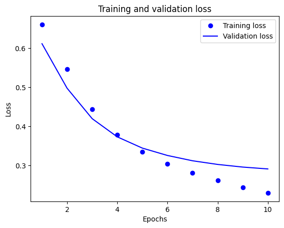
plt.plot(epochs, loss, 'bo', label='Training loss')
# b is for "solid blue line"
plt.plot(epochs, val_loss, 'b', label='Validation loss')
plt.title('Training and validation loss')
plt.xlabel('Epochs')
plt.ylabel('Loss')
plt.legend()
plt.show()
plt.plot(epochs, acc, 'bo', label='Training acc')
plt.plot(epochs, val_acc, 'b', label='Validation acc')
plt.title('Training and validation accuracy')
plt.xlabel('Epochs')
plt.ylabel('Accuracy')
plt.legend(loc='lower right')

plt.show()
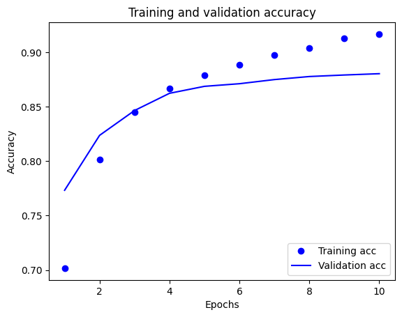
このグラフでは、点はトレーニングの損失と正解度を表し、実線は検証の損失と正解度を表します。
トレーニングの損失がエポックごとに下降し、トレーニングの正解度がエポックごとに上昇していることに注目してください。これは、勾配下降最適化を使用しているときに見られる現象で、イテレーションごとに希望する量を最小化します。
これは検証の損失と精度には当てはまりません。これらはトレーニング精度の前にピークに達しているようです。これが過適合の例で、モデルが、遭遇したことのないデータよりもトレーニングデータで優れたパフォーマンスを発揮する現象です。この後、モデルは過度に最適化し、テストデータに一般化しないトレーニングデータ特有の表現を学習します。
この特定のケースでは、検証の正解度が向上しなくなったときにトレーニングを停止することにより、過適合を防ぐことができます。これを行うには、tf.keras.callbacks.EarlyStopping コールバックを使用することができます。
モデルをエクスポートする
上記のコードでは、モデルにテキストをフィードする前に、TextVectorization レイヤーをデータセットに適用しました。モデルで生の文字列を処理できるようにする場合 (たとえば、展開を簡素化するため)、モデル内に TextVectorization レイヤーを含めることができます。これを行うには、トレーニングしたばかりの重みを使用して新しいモデルを作成します。
export_model = tf.keras.Sequential([
  vectorize_layer,
  model,
  layers.Activation('sigmoid')
])

export_model.compile(
    loss=losses.BinaryCrossentropy(from_logits=False), optimizer="adam", metrics=['accuracy']
)

# Test it with `raw_test_ds`, which yields raw strings
loss, accuracy = export_model.evaluate(raw_test_ds)
print(accuracy)
782/782 [==============================] - 3s 4ms/step - loss: 0.3099 - accuracy: 0.8734
0.8733999729156494
新しいデータの推論
新しい例の予測を取得するには、model.predict()を呼び出します。
examples = [
  "The movie was great!",
  "The movie was okay.",
  "The movie was terrible..."
]

export_model.predict(examples)
1/1 [==============================] - 0s 175ms/step
array([[0.61918825],
       [0.44328377],
       [0.3598296 ]], dtype=float32)
モデル内にテキスト前処理ロジックを含めると、モデルを本番環境にエクスポートして展開を簡素化し、トレーニング/テストスキューの可能性を減らすことができます。
TextVectorization レイヤーを適用する場所を選択する際に性能の違いに留意する必要があります。モデルの外部で使用すると、GPU でトレーニングするときに非同期 CPU 処理とデータのバッファリングを行うことができます。したがって、GPU でモデルをトレーニングしている場合は、モデルの開発中に最高のパフォーマンスを得るためにこのオプションを使用し、デプロイの準備ができたらモデル内に TextVectorization レイヤーを含めるように切り替えることをお勧めします。
モデルの保存の詳細については、このチュートリアルにアクセスしてください。
演習:StackOverflow の質問に対するマルチクラス分類
このチュートリアルでは、IMDB データセットで二項分類器を最初からトレーニングする方法を示しました。演習として、このノートブックを変更して、Stack Overflow のプログラミング質問のタグを予測するマルチクラス分類器をトレーニングできます。
Stack Overflow に投稿された数千のプログラミングに関する質問(たとえば、「Python でディクショナリを値で並べ替える方法」)の本文を含むデータセットが用意されています。それぞれ、1 つのタグ(Python、CSharp、JavaScript、または Java のいずれか)でラベル付けされています。この演習では、質問を入力として受け取り、適切なタグ(この場合は Python)を予測します。
使用するデータセットには、1,700 万件以上の投稿を含む BigQuery の大規模な StackOverflow パブリックデータセットから抽出された数千の質問が含まれています。
データセットをダウンロードすると、以前に使用した IMDB データセットと同様のディレクトリ構造になっていることがわかります。
train/
...python/
......0.txt
......1.txt
...javascript/
......0.txt
......1.txt
...csharp/
......0.txt
......1.txt
...java/
......0.txt
......1.txt
注意: 分類問題の難易度を上げるために、プログラミングの質問での Python、CSharp、JavaScript、または Java という単語は、blank という単語に置き換えられました(多くの質問には、対象の言語が含まれているため)。
この演習を完了するには、、このノートブックを変更してStackOverflow データセットを操作する必要があります。次の変更を行います。
ノートブックの上部で、IMDB データセットをダウンロードするコードを、事前に準備されている Stack Overflow データセットをダウンロードするコードで更新します。Stack Overflow データセットは同様のディレクトリ構造を持っているため、多くの変更を加える必要はありません。
4 つの出力クラスがあるため、モデルの最後のレイヤーを
Dense(4)に変更します。モデルをコンパイルするときは、損失を
tf.keras.losses.SparseCategoricalCrossentropy(from_logits=True)に変更します。これは、各クラスのラベルが整数である場合に、マルチクラス分類問題に使用する正しい損失関数です。(この場合、 0、1、2、または 3 のいずれかになります)。さらに、これはマルチクラス分類の問題であるため、メトリックをmetrics=['accuracy']に変更します (tf.metrics.BinaryAccuracyはバイナリ分類器にのみ使用されます)。経時的な精度をプロットする場合は、
binary_accuracyおよびval_binary_accuracyをそれぞれaccuracyおよびval_accuracyに変更します。これらの変更が完了すると、マルチクラス分類器をトレーニングできるようになります。
詳細
このチュートリアルでは、最初からテキスト分類を実行する方法を紹介しました。一般的なテキスト分類ワークフローの詳細については、Google Developers のテキスト分類ガイドをご覧ください。
# MIT License
#
# Copyright (c) 2017 François Chollet
#
# Permission is hereby granted, free of charge, to any person obtaining a
# copy of this software and associated documentation files (the "Software"),
# to deal in the Software without restriction, including without limitation
# the rights to use, copy, modify, merge, publish, distribute, sublicense,
# and/or sell copies of the Software, and to permit persons to whom the
# Software is furnished to do so, subject to the following conditions:
#
# The above copyright notice and this permission notice shall be included in
# all copies or substantial portions of the Software.
#
# THE SOFTWARE IS PROVIDED "AS IS", WITHOUT WARRANTY OF ANY KIND, EXPRESS OR
# IMPLIED, INCLUDING BUT NOT LIMITED TO THE WARRANTIES OF MERCHANTABILITY,
# FITNESS FOR A PARTICULAR PURPOSE AND NONINFRINGEMENT. IN NO EVENT SHALL
# THE AUTHORS OR COPYRIGHT HOLDERS BE LIABLE FOR ANY CLAIM, DAMAGES OR OTHER
# LIABILITY, WHETHER IN AN ACTION OF CONTRACT, TORT OR OTHERWISE, ARISING
# FROM, OUT OF OR IN CONNECTION WITH THE SOFTWARE OR THE USE OR OTHER
# DEALINGS IN THE SOFTWARE.