
|
|
|
 View on GitHub View on GitHub
|
|
In this colab, you will learn how to inspect and create the structure of a model directly. We assume you are familiar with the concepts introduced in the beginner and intermediate colabs.
In this colab, you will:
Train a Random Forest model and access its structure programmatically.
Create a Random Forest model by hand and use it as a classical model.
Setup
# Install TensorFlow Decision Forests.pip install tensorflow_decision_forests# Use wurlitzer to show the training logs.pip install wurlitzer
import os
# Keep using Keras 2
os.environ['TF_USE_LEGACY_KERAS'] = '1'

import tensorflow_decision_forests as tfdf

import numpy as np
import pandas as pd
import tensorflow as tf
import tf_keras
import matplotlib.pyplot as plt
import math
import collections
2026-01-12 14:08:35.487684: E external/local_xla/xla/stream_executor/cuda/cuda_fft.cc:467] Unable to register cuFFT factory: Attempting to register factory for plugin cuFFT when one has already been registered
WARNING: All log messages before absl::InitializeLog() is called are written to STDERR
E0000 00:00:1768226915.510047  150155 cuda_dnn.cc:8579] Unable to register cuDNN factory: Attempting to register factory for plugin cuDNN when one has already been registered
E0000 00:00:1768226915.517716  150155 cuda_blas.cc:1407] Unable to register cuBLAS factory: Attempting to register factory for plugin cuBLAS when one has already been registered
W0000 00:00:1768226915.536150  150155 computation_placer.cc:177] computation placer already registered. Please check linkage and avoid linking the same target more than once.
W0000 00:00:1768226915.536175  150155 computation_placer.cc:177] computation placer already registered. Please check linkage and avoid linking the same target more than once.
W0000 00:00:1768226915.536178  150155 computation_placer.cc:177] computation placer already registered. Please check linkage and avoid linking the same target more than once.
W0000 00:00:1768226915.536180  150155 computation_placer.cc:177] computation placer already registered. Please check linkage and avoid linking the same target more than once.
The hidden code cell limits the output height in colab.
from IPython.core.magic import register_line_magic
from IPython.display import Javascript
from IPython.display import display as ipy_display

# Some of the model training logs can cover the full
# screen if not compressed to a smaller viewport.
# This magic allows setting a max height for a cell.
@register_line_magic
def set_cell_height(size):
  ipy_display(
      Javascript("google.colab.output.setIframeHeight(0, true, {maxHeight: " +
                 str(size) + "})"))
Train a simple Random Forest
We train a Random Forest like in the beginner colab:
# Download the dataset
!wget -q https://storage.googleapis.com/download.tensorflow.org/data/palmer_penguins/penguins.csv -O /tmp/penguins.csv

# Load a dataset into a Pandas Dataframe.
dataset_df = pd.read_csv("/tmp/penguins.csv")

# Show the first three examples.
print(dataset_df.head(3))

# Convert the pandas dataframe into a tf dataset.
dataset_tf = tfdf.keras.pd_dataframe_to_tf_dataset(dataset_df, label="species")

# Train the Random Forest
model = tfdf.keras.RandomForestModel(compute_oob_variable_importances=True)
model.fit(x=dataset_tf)
species     island  bill_length_mm  bill_depth_mm  flipper_length_mm  \
0  Adelie  Torgersen            39.1           18.7              181.0
1  Adelie  Torgersen            39.5           17.4              186.0
2  Adelie  Torgersen            40.3           18.0              195.0

   body_mass_g     sex  year
0       3750.0    male  2007
1       3800.0  female  2007
2       3250.0  female  2007
Warning: The `num_threads` constructor argument is not set and the number of CPU is os.cpu_count()=32 > 32. Setting num_threads to 32. Set num_threads manually to use more than 32 cpus.
I0000 00:00:1768226920.022534  150155 gpu_device.cc:2019] Created device /job:localhost/replica:0/task:0/device:GPU:0 with 13638 MB memory:  -> device: 0, name: Tesla T4, pci bus id: 0000:00:05.0, compute capability: 7.5
I0000 00:00:1768226920.024914  150155 gpu_device.cc:2019] Created device /job:localhost/replica:0/task:0/device:GPU:1 with 13756 MB memory:  -> device: 1, name: Tesla T4, pci bus id: 0000:00:06.0, compute capability: 7.5
I0000 00:00:1768226920.027104  150155 gpu_device.cc:2019] Created device /job:localhost/replica:0/task:0/device:GPU:2 with 13756 MB memory:  -> device: 2, name: Tesla T4, pci bus id: 0000:00:07.0, compute capability: 7.5
I0000 00:00:1768226920.029256  150155 gpu_device.cc:2019] Created device /job:localhost/replica:0/task:0/device:GPU:3 with 13756 MB memory:  -> device: 3, name: Tesla T4, pci bus id: 0000:00:08.0, compute capability: 7.5
WARNING:absl:The `num_threads` constructor argument is not set and the number of CPU is os.cpu_count()=32 > 32. Setting num_threads to 32. Set num_threads manually to use more than 32 cpus.
Use /tmpfs/tmp/tmp1133vua7 as temporary training directory
Reading training dataset...
Training dataset read in 0:00:03.771078. Found 344 examples.
Training model...
Model trained in 0:00:00.097883
Compiling model...
WARNING: All log messages before absl::InitializeLog() is called are written to STDERR
I0000 00:00:1768226924.178818  150155 kernel.cc:782] Start Yggdrasil model training
I0000 00:00:1768226924.178870  150155 kernel.cc:783] Collect training examples
I0000 00:00:1768226924.178879  150155 kernel.cc:795] Dataspec guide:
column_guides {
  column_name_pattern: "^__LABEL$"
  type: CATEGORICAL
  categorial {
    min_vocab_frequency: 0
    max_vocab_count: -1
  }
}
default_column_guide {
  categorial {
    max_vocab_count: 2000
  }
  discretized_numerical {
    maximum_num_bins: 255
  }
}
ignore_columns_without_guides: false
detect_numerical_as_discretized_numerical: false

I0000 00:00:1768226924.179251  150155 kernel.cc:401] Number of batches: 1
I0000 00:00:1768226924.179269  150155 kernel.cc:402] Number of examples: 344
I0000 00:00:1768226924.179368  150155 kernel.cc:802] Training dataset:
Number of records: 344
Number of columns: 8

Number of columns by type:
    NUMERICAL: 5 (62.5%)
    CATEGORICAL: 3 (37.5%)

Columns:

NUMERICAL: 5 (62.5%)
    1: "bill_depth_mm" NUMERICAL num-nas:2 (0.581395%) mean:17.1512 min:13.1 max:21.5 sd:1.9719
    2: "bill_length_mm" NUMERICAL num-nas:2 (0.581395%) mean:43.9219 min:32.1 max:59.6 sd:5.4516
    3: "body_mass_g" NUMERICAL num-nas:2 (0.581395%) mean:4201.75 min:2700 max:6300 sd:800.781
    4: "flipper_length_mm" NUMERICAL num-nas:2 (0.581395%) mean:200.915 min:172 max:231 sd:14.0411
    7: "year" NUMERICAL mean:2008.03 min:2007 max:2009 sd:0.817166

CATEGORICAL: 3 (37.5%)
    0: "__LABEL" CATEGORICAL integerized vocab-size:4 no-ood-item
    5: "island" CATEGORICAL has-dict vocab-size:4 zero-ood-items most-frequent:"Biscoe" 168 (48.8372%)
    6: "sex" CATEGORICAL num-nas:11 (3.19767%) has-dict vocab-size:3 zero-ood-items most-frequent:"male" 168 (50.4505%)

Terminology:
    nas: Number of non-available (i.e. missing) values.
    ood: Out of dictionary.
    manually-defined: Attribute whose type is manually defined by the user, i.e., the type was not automatically inferred.
    tokenized: The attribute value is obtained through tokenization.
    has-dict: The attribute is attached to a string dictionary e.g. a categorical attribute stored as a string.
    vocab-size: Number of unique values.

I0000 00:00:1768226924.179391  150155 kernel.cc:818] Configure learner
I0000 00:00:1768226924.179572  150155 kernel.cc:831] Training config:
learner: "RANDOM_FOREST"
features: "^bill_depth_mm$"
features: "^bill_length_mm$"
features: "^body_mass_g$"
features: "^flipper_length_mm$"
features: "^island$"
features: "^sex$"
features: "^year$"
label: "^__LABEL$"
task: CLASSIFICATION
random_seed: 123456
metadata {
  framework: "TF Keras"
}
pure_serving_model: false
[yggdrasil_decision_forests.model.random_forest.proto.random_forest_config] {
  num_trees: 300
  decision_tree {
    max_depth: 16
    min_examples: 5
    in_split_min_examples_check: true
    keep_non_leaf_label_distribution: true
    num_candidate_attributes: 0
    missing_value_policy: GLOBAL_IMPUTATION
    allow_na_conditions: false
    categorical_set_greedy_forward {
      sampling: 0.1
      max_num_items: -1
      min_item_frequency: 1
    }
    growing_strategy_local {
    }
    categorical {
      cart {
      }
    }
    axis_aligned_split {
    }
    internal {
      sorting_strategy: PRESORTED
    }
    uplift {
      min_examples_in_treatment: 5
      split_score: KULLBACK_LEIBLER
    }
    numerical_vector_sequence {
      max_num_test_examples: 1000
      num_random_selected_anchors: 100
    }
  }
  winner_take_all_inference: true
  compute_oob_performances: true
  compute_oob_variable_importances: true
  num_oob_variable_importances_permutations: 1
  bootstrap_training_dataset: true
  bootstrap_size_ratio: 1
  adapt_bootstrap_size_ratio_for_maximum_training_duration: false
  sampling_with_replacement: true
}

I0000 00:00:1768226924.179932  150155 kernel.cc:834] Deployment config:
cache_path: "/tmpfs/tmp/tmp1133vua7/working_cache"
num_threads: 32
try_resume_training: true

I0000 00:00:1768226924.180042  150380 kernel.cc:895] Train model
I0000 00:00:1768226924.180148  150380 random_forest.cc:438] Training random forest on 344 example(s) and 7 feature(s).
I0000 00:00:1768226924.184195  150380 gpu.cc:93] Cannot initialize GPU: Not compiled with GPU support
I0000 00:00:1768226924.186044  150389 random_forest.cc:865] Train tree 1/300 accuracy:0.944882 logloss:1.98666 [index:2 total:0.00s tree:0.00s]
I0000 00:00:1768226924.186216  150398 random_forest.cc:865] Train tree 11/300 accuracy:0.945813 logloss:1.77896 [index:10 total:0.00s tree:0.00s]
I0000 00:00:1768226924.186533  150409 random_forest.cc:865] Train tree 24/300 accuracy:0.965986 logloss:0.76054 [index:23 total:0.00s tree:0.00s]
I0000 00:00:1768226924.186858  150414 random_forest.cc:865] Train tree 34/300 accuracy:0.965732 logloss:0.477947 [index:29 total:0.00s tree:0.00s]
I0000 00:00:1768226924.188161  150399 random_forest.cc:865] Train tree 45/300 accuracy:0.965116 logloss:0.578036 [index:44 total:0.00s tree:0.00s]
I0000 00:00:1768226924.190016  150408 random_forest.cc:865] Train tree 55/300 accuracy:0.97093 logloss:0.376297 [index:54 total:0.01s tree:0.00s]
I0000 00:00:1768226924.191278  150415 random_forest.cc:865] Train tree 65/300 accuracy:0.97093 logloss:0.378839 [index:64 total:0.01s tree:0.00s]
I0000 00:00:1768226924.193038  150393 random_forest.cc:865] Train tree 77/300 accuracy:0.973837 logloss:0.275567 [index:76 total:0.01s tree:0.00s]
I0000 00:00:1768226924.196059  150416 random_forest.cc:865] Train tree 98/300 accuracy:0.976744 logloss:0.17131 [index:97 total:0.01s tree:0.00s]
I0000 00:00:1768226924.197309  150417 random_forest.cc:865] Train tree 108/300 accuracy:0.976744 logloss:0.166666 [index:107 total:0.01s tree:0.00s]
I0000 00:00:1768226924.199854  150419 random_forest.cc:865] Train tree 125/300 accuracy:0.976744 logloss:0.0725837 [index:124 total:0.02s tree:0.00s]
I0000 00:00:1768226924.201389  150416 random_forest.cc:865] Train tree 136/300 accuracy:0.976744 logloss:0.0721071 [index:135 total:0.02s tree:0.00s]
I0000 00:00:1768226924.203526  150402 random_forest.cc:865] Train tree 150/300 accuracy:0.976744 logloss:0.0716672 [index:149 total:0.02s tree:0.00s]
I0000 00:00:1768226924.205494  150418 random_forest.cc:865] Train tree 163/300 accuracy:0.976744 logloss:0.0723785 [index:162 total:0.02s tree:0.00s]
I0000 00:00:1768226924.206989  150395 random_forest.cc:865] Train tree 173/300 accuracy:0.976744 logloss:0.0718518 [index:172 total:0.02s tree:0.00s]
I0000 00:00:1768226924.208726  150402 random_forest.cc:865] Train tree 184/300 accuracy:0.976744 logloss:0.0708714 [index:183 total:0.02s tree:0.00s]
I0000 00:00:1768226924.210282  150413 random_forest.cc:865] Train tree 194/300 accuracy:0.976744 logloss:0.0697211 [index:193 total:0.03s tree:0.00s]
I0000 00:00:1768226924.211915  150393 random_forest.cc:865] Train tree 204/300 accuracy:0.976744 logloss:0.0684952 [index:203 total:0.03s tree:0.00s]
I0000 00:00:1768226924.213450  150411 random_forest.cc:865] Train tree 215/300 accuracy:0.976744 logloss:0.0681587 [index:214 total:0.03s tree:0.00s]
I0000 00:00:1768226924.215064  150388 random_forest.cc:865] Train tree 225/300 accuracy:0.976744 logloss:0.0688663 [index:224 total:0.03s tree:0.00s]
I0000 00:00:1768226924.216633  150409 random_forest.cc:865] Train tree 237/300 accuracy:0.976744 logloss:0.068661 [index:236 total:0.03s tree:0.00s]
I0000 00:00:1768226924.218987  150408 random_forest.cc:865] Train tree 251/300 accuracy:0.976744 logloss:0.0680787 [index:250 total:0.03s tree:0.00s]
I0000 00:00:1768226924.221144  150390 random_forest.cc:865] Train tree 267/300 accuracy:0.976744 logloss:0.0685897 [index:266 total:0.04s tree:0.00s]
I0000 00:00:1768226924.223877  150394 random_forest.cc:865] Train tree 287/300 accuracy:0.976744 logloss:0.0681651 [index:286 total:0.04s tree:0.00s]
I0000 00:00:1768226924.225839  150395 random_forest.cc:865] Train tree 300/300 accuracy:0.976744 logloss:0.0676584 [index:299 total:0.04s tree:0.00s]
I0000 00:00:1768226924.231081  150380 random_forest.cc:949] Final OOB metrics: accuracy:0.976744 logloss:0.0676584
I0000 00:00:1768226924.232352  150380 feature_importance.cc:196] Running 8 features on 32 threads with 1 rounds
I0000 00:00:1768226924.236343  150380 kernel.cc:926] Export model in log directory: /tmpfs/tmp/tmp1133vua7 with prefix f016df2d741d4761
I0000 00:00:1768226924.239996  150380 kernel.cc:944] Save model in resources
I0000 00:00:1768226924.242495  150155 abstract_model.cc:921] Model self evaluation:
Number of predictions (without weights): 344
Number of predictions (with weights): 344
Task: CLASSIFICATION
Label: __LABEL

Accuracy: 0.976744  CI95[W][0.958431 0.988377]
LogLoss: : 0.0676584
ErrorRate: : 0.0232558

Default Accuracy: : 0.44186
Default LogLoss: : 1.04916
Default ErrorRate: : 0.55814

Confusion Table:
truth\prediction
     1   2    3
1  148   3    1
2    2  66    0
3    2   0  122
Total: 344


WARNING: All log messages before absl::InitializeLog() is called are written to STDERR
I0000 00:00:1768226924.267848  150155 decision_forest.cc:808] Model loaded with 300 root(s), 5080 node(s), and 7 input feature(s).
I0000 00:00:1768226924.271050  150155 abstract_model.cc:1439] Engine "RandomForestGeneric" built
Model compiled.
<tf_keras.src.callbacks.History at 0x7fed709d28b0>
Note the compute_oob_variable_importances=True
hyper-parameter in the model constructor. This option computes the Out-of-bag (OOB)
variable importance during training. This is a popular
permutation variable importance for Random Forest models.
Computing the OOB Variable importance does not impact the final model, it will slow the training on large datasets.
Check the model summary:
%set_cell_height 300

model.summary()
<IPython.core.display.Javascript object>
Model: "random_forest_model"
_________________________________________________________________
 Layer (type)                Output Shape              Param #
=================================================================
=================================================================
Total params: 1 (1.00 Byte)
Trainable params: 0 (0.00 Byte)
Non-trainable params: 1 (1.00 Byte)
_________________________________________________________________
Type: "RANDOM_FOREST"
Task: CLASSIFICATION
Label: "__LABEL"

Input Features (7):
    bill_depth_mm
    bill_length_mm
    body_mass_g
    flipper_length_mm
    island
    sex
    year

No weights

Variable Importance: INV_MEAN_MIN_DEPTH:

    1. "flipper_length_mm"  0.440513 ################
    2.    "bill_length_mm"  0.438028 ###############
    3.     "bill_depth_mm"  0.299751 #####
    4.            "island"  0.295079 #####
    5.       "body_mass_g"  0.256534 ##
    6.               "sex"  0.225708
    7.              "year"  0.224020

Variable Importance: MEAN_DECREASE_IN_ACCURACY:

    1.    "bill_length_mm"  0.151163 ################
    2.            "island"  0.008721 #
    3.     "bill_depth_mm"  0.000000
    4.       "body_mass_g"  0.000000
    5.               "sex"  0.000000
    6.              "year"  0.000000
    7. "flipper_length_mm" -0.002907

Variable Importance: MEAN_DECREASE_IN_AP_1_VS_OTHERS:

    1.    "bill_length_mm"  0.083305 ################
    2.            "island"  0.007664 #
    3. "flipper_length_mm"  0.003400
    4.     "bill_depth_mm"  0.002741
    5.       "body_mass_g"  0.000722
    6.               "sex"  0.000644
    7.              "year"  0.000000

Variable Importance: MEAN_DECREASE_IN_AP_2_VS_OTHERS:

    1.    "bill_length_mm"  0.508510 ################
    2.            "island"  0.023487
    3.     "bill_depth_mm"  0.007744
    4. "flipper_length_mm"  0.006008
    5.       "body_mass_g"  0.003017
    6.               "sex"  0.001537
    7.              "year" -0.000245

Variable Importance: MEAN_DECREASE_IN_AP_3_VS_OTHERS:

    1.            "island"  0.002192 ################
    2.    "bill_length_mm"  0.001572 ############
    3.     "bill_depth_mm"  0.000497 #######
    4.               "sex"  0.000000 ####
    5.              "year"  0.000000 ####
    6.       "body_mass_g" -0.000053 ####
    7. "flipper_length_mm" -0.000890

Variable Importance: MEAN_DECREASE_IN_AUC_1_VS_OTHERS:

    1.    "bill_length_mm"  0.071306 ################
    2.            "island"  0.007299 #
    3. "flipper_length_mm"  0.004506 #
    4.     "bill_depth_mm"  0.002124
    5.       "body_mass_g"  0.000548
    6.               "sex"  0.000480
    7.              "year"  0.000000

Variable Importance: MEAN_DECREASE_IN_AUC_2_VS_OTHERS:

    1.    "bill_length_mm"  0.108642 ################
    2.            "island"  0.014493 ##
    3.     "bill_depth_mm"  0.007406 #
    4. "flipper_length_mm"  0.005195
    5.       "body_mass_g"  0.001012
    6.               "sex"  0.000480
    7.              "year" -0.000053

Variable Importance: MEAN_DECREASE_IN_AUC_3_VS_OTHERS:

    1.            "island"  0.002126 ################
    2.    "bill_length_mm"  0.001393 ###########
    3.     "bill_depth_mm"  0.000293 #####
    4.               "sex"  0.000000 ###
    5.              "year"  0.000000 ###
    6.       "body_mass_g" -0.000037 ###
    7. "flipper_length_mm" -0.000550

Variable Importance: MEAN_DECREASE_IN_PRAUC_1_VS_OTHERS:

    1.    "bill_length_mm"  0.083122 ################
    2.            "island"  0.010887 ##
    3. "flipper_length_mm"  0.003425
    4.     "bill_depth_mm"  0.002731
    5.       "body_mass_g"  0.000719
    6.               "sex"  0.000641
    7.              "year"  0.000000

Variable Importance: MEAN_DECREASE_IN_PRAUC_2_VS_OTHERS:

    1.    "bill_length_mm"  0.497611 ################
    2.            "island"  0.024045
    3.     "bill_depth_mm"  0.007734
    4. "flipper_length_mm"  0.006017
    5.       "body_mass_g"  0.003000
    6.               "sex"  0.001528
    7.              "year" -0.000243

Variable Importance: MEAN_DECREASE_IN_PRAUC_3_VS_OTHERS:

    1.            "island"  0.002187 ################
    2.    "bill_length_mm"  0.001568 ############
    3.     "bill_depth_mm"  0.000495 #######
    4.               "sex"  0.000000 ####
    5.              "year"  0.000000 ####
    6.       "body_mass_g" -0.000053 ####
    7. "flipper_length_mm" -0.000886

Variable Importance: NUM_AS_ROOT:

    1. "flipper_length_mm" 157.000000 ################
    2.    "bill_length_mm" 76.000000 #######
    3.     "bill_depth_mm" 52.000000 #####
    4.            "island" 12.000000
    5.       "body_mass_g"  3.000000

Variable Importance: NUM_NODES:

    1.    "bill_length_mm" 778.000000 ################
    2.     "bill_depth_mm" 463.000000 #########
    3. "flipper_length_mm" 414.000000 ########
    4.            "island" 342.000000 ######
    5.       "body_mass_g" 338.000000 ######
    6.               "sex" 36.000000
    7.              "year" 19.000000

Variable Importance: SUM_SCORE:

    1.    "bill_length_mm" 36515.793787 ################
    2. "flipper_length_mm" 35120.434174 ###############
    3.            "island" 14669.408395 ######
    4.     "bill_depth_mm" 14515.446617 ######
    5.       "body_mass_g" 3485.330881 #
    6.               "sex" 354.201073
    7.              "year" 49.737758


Winner takes all: true
Out-of-bag evaluation: accuracy:0.976744 logloss:0.0676584
Number of trees: 300
Total number of nodes: 5080

Number of nodes by tree:
Count: 300 Average: 16.9333 StdDev: 3.10197
Min: 11 Max: 31 Ignored: 0
----------------------------------------------
[ 11, 12)  6   2.00%   2.00% #
[ 12, 13)  0   0.00%   2.00%
[ 13, 14) 46  15.33%  17.33% #####
[ 14, 15)  0   0.00%  17.33%
[ 15, 16) 70  23.33%  40.67% ########
[ 16, 17)  0   0.00%  40.67%
[ 17, 18) 84  28.00%  68.67% ##########
[ 18, 19)  0   0.00%  68.67%
[ 19, 20) 46  15.33%  84.00% #####
[ 20, 21)  0   0.00%  84.00%
[ 21, 22) 30  10.00%  94.00% ####
[ 22, 23)  0   0.00%  94.00%
[ 23, 24) 13   4.33%  98.33% ##
[ 24, 25)  0   0.00%  98.33%
[ 25, 26)  2   0.67%  99.00%
[ 26, 27)  0   0.00%  99.00%
[ 27, 28)  2   0.67%  99.67%
[ 28, 29)  0   0.00%  99.67%
[ 29, 30)  0   0.00%  99.67%
[ 30, 31]  1   0.33% 100.00%

Depth by leafs:
Count: 2690 Average: 3.53271 StdDev: 1.06789
Min: 2 Max: 7 Ignored: 0
----------------------------------------------
[ 2, 3) 545  20.26%  20.26% ######
[ 3, 4) 747  27.77%  48.03% ########
[ 4, 5) 888  33.01%  81.04% ##########
[ 5, 6) 444  16.51%  97.55% #####
[ 6, 7)  62   2.30%  99.85% #
[ 7, 7]   4   0.15% 100.00%

Number of training obs by leaf:
Count: 2690 Average: 38.3643 StdDev: 44.8651
Min: 5 Max: 155 Ignored: 0
----------------------------------------------
[   5,  12) 1474  54.80%  54.80% ##########
[  12,  20)  124   4.61%  59.41% #
[  20,  27)   48   1.78%  61.19%
[  27,  35)   74   2.75%  63.94% #
[  35,  42)   58   2.16%  66.10%
[  42,  50)   85   3.16%  69.26% #
[  50,  57)   96   3.57%  72.83% #
[  57,  65)   87   3.23%  76.06% #
[  65,  72)   49   1.82%  77.88%
[  72,  80)   23   0.86%  78.74%
[  80,  88)   30   1.12%  79.85%
[  88,  95)   23   0.86%  80.71%
[  95, 103)   42   1.56%  82.27%
[ 103, 110)   62   2.30%  84.57%
[ 110, 118)  115   4.28%  88.85% #
[ 118, 125)  115   4.28%  93.12% #
[ 125, 133)   98   3.64%  96.77% #
[ 133, 140)   49   1.82%  98.59%
[ 140, 148)   31   1.15%  99.74%
[ 148, 155]    7   0.26% 100.00%

Attribute in nodes:
    778 : bill_length_mm [NUMERICAL]
    463 : bill_depth_mm [NUMERICAL]
    414 : flipper_length_mm [NUMERICAL]
    342 : island [CATEGORICAL]
    338 : body_mass_g [NUMERICAL]
    36 : sex [CATEGORICAL]
    19 : year [NUMERICAL]

Attribute in nodes with depth <= 0:
    157 : flipper_length_mm [NUMERICAL]
    76 : bill_length_mm [NUMERICAL]
    52 : bill_depth_mm [NUMERICAL]
    12 : island [CATEGORICAL]
    3 : body_mass_g [NUMERICAL]

Attribute in nodes with depth <= 1:
    250 : bill_length_mm [NUMERICAL]
    244 : flipper_length_mm [NUMERICAL]
    183 : bill_depth_mm [NUMERICAL]
    170 : island [CATEGORICAL]
    53 : body_mass_g [NUMERICAL]

Attribute in nodes with depth <= 2:
    462 : bill_length_mm [NUMERICAL]
    320 : flipper_length_mm [NUMERICAL]
    310 : bill_depth_mm [NUMERICAL]
    287 : island [CATEGORICAL]
    162 : body_mass_g [NUMERICAL]
    9 : sex [CATEGORICAL]
    5 : year [NUMERICAL]

Attribute in nodes with depth <= 3:
    669 : bill_length_mm [NUMERICAL]
    410 : bill_depth_mm [NUMERICAL]
    383 : flipper_length_mm [NUMERICAL]
    328 : island [CATEGORICAL]
    286 : body_mass_g [NUMERICAL]
    32 : sex [CATEGORICAL]
    10 : year [NUMERICAL]

Attribute in nodes with depth <= 5:
    778 : bill_length_mm [NUMERICAL]
    462 : bill_depth_mm [NUMERICAL]
    413 : flipper_length_mm [NUMERICAL]
    342 : island [CATEGORICAL]
    338 : body_mass_g [NUMERICAL]
    36 : sex [CATEGORICAL]
    19 : year [NUMERICAL]

Condition type in nodes:
    2012 : HigherCondition
    378 : ContainsBitmapCondition
Condition type in nodes with depth <= 0:
    288 : HigherCondition
    12 : ContainsBitmapCondition
Condition type in nodes with depth <= 1:
    730 : HigherCondition
    170 : ContainsBitmapCondition
Condition type in nodes with depth <= 2:
    1259 : HigherCondition
    296 : ContainsBitmapCondition
Condition type in nodes with depth <= 3:
    1758 : HigherCondition
    360 : ContainsBitmapCondition
Condition type in nodes with depth <= 5:
    2010 : HigherCondition
    378 : ContainsBitmapCondition
Node format: NOT_SET

Training OOB:
    trees: 1, Out-of-bag evaluation: accuracy:0.944882 logloss:1.98666
    trees: 11, Out-of-bag evaluation: accuracy:0.945813 logloss:1.77896
    trees: 24, Out-of-bag evaluation: accuracy:0.965986 logloss:0.76054
    trees: 34, Out-of-bag evaluation: accuracy:0.965732 logloss:0.477947
    trees: 45, Out-of-bag evaluation: accuracy:0.965116 logloss:0.578036
    trees: 55, Out-of-bag evaluation: accuracy:0.97093 logloss:0.376297
    trees: 65, Out-of-bag evaluation: accuracy:0.97093 logloss:0.378839
    trees: 77, Out-of-bag evaluation: accuracy:0.973837 logloss:0.275567
    trees: 98, Out-of-bag evaluation: accuracy:0.976744 logloss:0.17131
    trees: 108, Out-of-bag evaluation: accuracy:0.976744 logloss:0.166666
    trees: 125, Out-of-bag evaluation: accuracy:0.976744 logloss:0.0725837
    trees: 136, Out-of-bag evaluation: accuracy:0.976744 logloss:0.0721071
    trees: 150, Out-of-bag evaluation: accuracy:0.976744 logloss:0.0716672
    trees: 163, Out-of-bag evaluation: accuracy:0.976744 logloss:0.0723785
    trees: 173, Out-of-bag evaluation: accuracy:0.976744 logloss:0.0718518
    trees: 184, Out-of-bag evaluation: accuracy:0.976744 logloss:0.0708714
    trees: 194, Out-of-bag evaluation: accuracy:0.976744 logloss:0.0697211
    trees: 204, Out-of-bag evaluation: accuracy:0.976744 logloss:0.0684952
    trees: 215, Out-of-bag evaluation: accuracy:0.976744 logloss:0.0681587
    trees: 225, Out-of-bag evaluation: accuracy:0.976744 logloss:0.0688663
    trees: 237, Out-of-bag evaluation: accuracy:0.976744 logloss:0.068661
    trees: 251, Out-of-bag evaluation: accuracy:0.976744 logloss:0.0680787
    trees: 267, Out-of-bag evaluation: accuracy:0.976744 logloss:0.0685897
    trees: 287, Out-of-bag evaluation: accuracy:0.976744 logloss:0.0681651
    trees: 300, Out-of-bag evaluation: accuracy:0.976744 logloss:0.0676584
Note the multiple variable importances with name MEAN_DECREASE_IN_*.
Plotting the model
Next, plot the model.
A Random Forest is a large model (this model has 300 trees and ~5k nodes; see the summary above). Therefore, only plot the first tree, and limit the nodes to depth 3.
tfdf.model_plotter.plot_model_in_colab(model, tree_idx=0, max_depth=3)
Inspect the model structure
The model structure and meta-data is
available through the inspector created by make_inspector().
inspector = model.make_inspector()
For our model, the available inspector fields are:
[field for field in dir(inspector) if not field.startswith("_")]
['MODEL_NAME',
 'dataspec',
 'directory',
 'evaluation',
 'export_to_tensorboard',
 'extract_all_trees',
 'extract_tree',
 'features',
 'file_prefix',
 'header',
 'iterate_on_nodes',
 'label',
 'label_classes',
 'metadata',
 'model_type',
 'num_trees',
 'objective',
 'specialized_header',
 'task',
 'training_logs',
 'tuning_logs',
 'variable_importances',
 'winner_take_all_inference']
Remember to see the API-reference or use ? for the builtin documentation.
?inspector.model_type
Some of the model meta-data:
print("Model type:", inspector.model_type())
print("Number of trees:", inspector.num_trees())
print("Objective:", inspector.objective())
print("Input features:", inspector.features())
Model type: RANDOM_FOREST
Number of trees: 300
Objective: Classification(label=__LABEL, class=None, num_classes=3)
Input features: ["bill_depth_mm" (1; #1), "bill_length_mm" (1; #2), "body_mass_g" (1; #3), "flipper_length_mm" (1; #4), "island" (4; #5), "sex" (4; #6), "year" (1; #7)]
evaluate() is the evaluation of the model computed during training. The dataset used for this evaluation depends on the algorithm. For example, it can be the validation dataset or the out-of-bag-dataset .
inspector.evaluation()
Evaluation(num_examples=344, accuracy=0.9767441860465116, loss=0.06765840018471313, rmse=None, ndcg=None, aucs=None, auuc=None, qini=None)
The variable importances are:
print(f"Available variable importances:")
for importance in inspector.variable_importances().keys():
  print("\t", importance)
Available variable importances:
     MEAN_DECREASE_IN_PRAUC_3_VS_OTHERS
     MEAN_DECREASE_IN_AP_2_VS_OTHERS
     MEAN_DECREASE_IN_AP_3_VS_OTHERS
     MEAN_DECREASE_IN_PRAUC_2_VS_OTHERS
     MEAN_DECREASE_IN_AP_1_VS_OTHERS
     NUM_AS_ROOT
     MEAN_DECREASE_IN_AUC_1_VS_OTHERS
     MEAN_DECREASE_IN_AUC_3_VS_OTHERS
     INV_MEAN_MIN_DEPTH
     MEAN_DECREASE_IN_ACCURACY
     NUM_NODES
     MEAN_DECREASE_IN_AUC_2_VS_OTHERS
     SUM_SCORE
     MEAN_DECREASE_IN_PRAUC_1_VS_OTHERS
Different variable importances have different semantics. For example, a feature
with a mean decrease in auc of 0.05 means that removing this feature from
the training dataset would reduce/hurt the AUC by 5%.
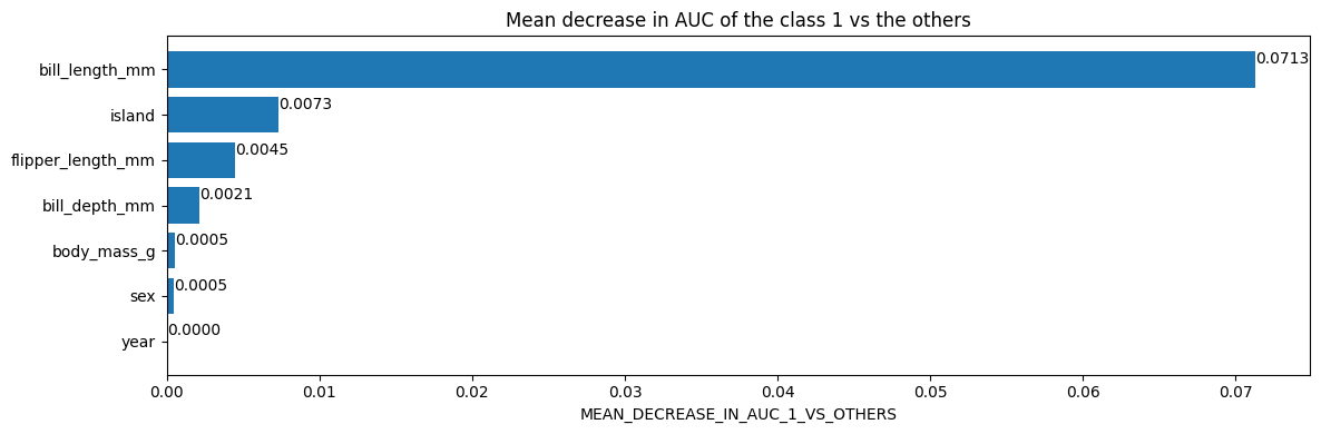
# Mean decrease in AUC of the class 1 vs the others.
inspector.variable_importances()["MEAN_DECREASE_IN_AUC_1_VS_OTHERS"]
[("bill_length_mm" (1; #2), 0.0713061951754389),
 ("island" (4; #5), 0.007298519736842035),
 ("flipper_length_mm" (1; #4), 0.004505893640351366),
 ("bill_depth_mm" (1; #1), 0.0021244517543865804),
 ("body_mass_g" (1; #3), 0.0005482456140351033),
 ("sex" (4; #6), 0.00047971491228060437),
 ("year" (1; #7), 0.0)]
Plot the variable importances from the inspector using Matplotlib
import matplotlib.pyplot as plt

plt.figure(figsize=(12, 4))

# Mean decrease in AUC of the class 1 vs the others.
variable_importance_metric = "MEAN_DECREASE_IN_AUC_1_VS_OTHERS"
variable_importances = inspector.variable_importances()[variable_importance_metric]

# Extract the feature name and importance values.
#
# `variable_importances` is a list of <feature, importance> tuples.
feature_names = [vi[0].name for vi in variable_importances]
feature_importances = [vi[1] for vi in variable_importances]
# The feature are ordered in decreasing importance value.
feature_ranks = range(len(feature_names))

bar = plt.barh(feature_ranks, feature_importances, label=[str(x) for x in feature_ranks])
plt.yticks(feature_ranks, feature_names)
plt.gca().invert_yaxis()

# TODO: Replace with "plt.bar_label()" when available.
# Label each bar with values
for importance, patch in zip(feature_importances, bar.patches):
  plt.text(patch.get_x() + patch.get_width(), patch.get_y(), f"{importance:.4f}", va="top")

plt.xlabel(variable_importance_metric)
plt.title("Mean decrease in AUC of the class 1 vs the others")
plt.tight_layout()
plt.show()
Finally, access the actual tree structure:
inspector.extract_tree(tree_idx=0)
Tree(root=NonLeafNode(condition=(bill_length_mm >= 43.25; miss=True, score=0.5482327342033386), pos_child=NonLeafNode(condition=(island in ['Biscoe']; miss=True, score=0.6515106558799744), pos_child=NonLeafNode(condition=(bill_depth_mm >= 17.225584030151367; miss=False, score=0.027205035090446472), pos_child=LeafNode(value=ProbabilityValue([0.16666666666666666, 0.0, 0.8333333333333334],n=6.0), idx=7), neg_child=LeafNode(value=ProbabilityValue([0.0, 0.0, 1.0],n=104.0), idx=6), value=ProbabilityValue([0.00909090909090909, 0.0, 0.990909090909091],n=110.0)), neg_child=LeafNode(value=ProbabilityValue([0.0, 1.0, 0.0],n=61.0), idx=5), value=ProbabilityValue([0.005847953216374269, 0.3567251461988304, 0.6374269005847953],n=171.0)), neg_child=NonLeafNode(condition=(bill_depth_mm >= 15.100000381469727; miss=True, score=0.150658518075943), pos_child=NonLeafNode(condition=(flipper_length_mm >= 187.5; miss=True, score=0.036139510571956635), pos_child=LeafNode(value=ProbabilityValue([1.0, 0.0, 0.0],n=104.0), idx=4), neg_child=NonLeafNode(condition=(bill_length_mm >= 42.30000305175781; miss=True, score=0.23430533707141876), pos_child=LeafNode(value=ProbabilityValue([0.0, 1.0, 0.0],n=5.0), idx=3), neg_child=NonLeafNode(condition=(bill_length_mm >= 40.55000305175781; miss=True, score=0.043961383402347565), pos_child=LeafNode(value=ProbabilityValue([0.8, 0.2, 0.0],n=5.0), idx=2), neg_child=LeafNode(value=ProbabilityValue([1.0, 0.0, 0.0],n=53.0), idx=1), value=ProbabilityValue([0.9827586206896551, 0.017241379310344827, 0.0],n=58.0)), value=ProbabilityValue([0.9047619047619048, 0.09523809523809523, 0.0],n=63.0)), value=ProbabilityValue([0.9640718562874252, 0.03592814371257485, 0.0],n=167.0)), neg_child=LeafNode(value=ProbabilityValue([0.0, 0.0, 1.0],n=6.0), idx=0), value=ProbabilityValue([0.930635838150289, 0.03468208092485549, 0.03468208092485549],n=173.0)), value=ProbabilityValue([0.47093023255813954, 0.19476744186046513, 0.33430232558139533],n=344.0)), label_classes=None)
Extracting a tree is not efficient. If speed is important, the model inspection can be done with the iterate_on_nodes() method instead. This method is a Depth First Pre-order traversals iterator on all the nodes of the model.
For following example computes how many times each feature is used (this is a kind of structural variable importance):
# number_of_use[F] will be the number of node using feature F in its condition.
number_of_use = collections.defaultdict(lambda: 0)

# Iterate over all the nodes in a Depth First Pre-order traversals.
for node_iter in inspector.iterate_on_nodes():

  if not isinstance(node_iter.node, tfdf.py_tree.node.NonLeafNode):
    # Skip the leaf nodes
    continue

  # Iterate over all the features used in the condition.
  # By default, models are "oblique" i.e. each node tests a single feature.
  for feature in node_iter.node.condition.features():
    number_of_use[feature] += 1

print("Number of condition nodes per features:")
for feature, count in number_of_use.items():
  print("\t", feature.name, ":", count)
Number of condition nodes per features:
     bill_length_mm : 778
     bill_depth_mm : 463
     flipper_length_mm : 414
     island : 342
     body_mass_g : 338
     year : 19
     sex : 36
Creating a model by hand
In this section you will create a small Random Forest model by hand. To make it extra easy, the model will only contain one simple tree:
3 label classes: Red, blue and green.
2 features: f1 (numerical) and f2 (string categorical)

f1>=1.5
    ├─(pos)─ f2 in ["cat","dog"]
    │         ├─(pos)─ value: [0.8, 0.1, 0.1]
    │         └─(neg)─ value: [0.1, 0.8, 0.1]
    └─(neg)─ value: [0.1, 0.1, 0.8]
# Create the model builder
builder = tfdf.builder.RandomForestBuilder(
    path="/tmp/manual_model",
    objective=tfdf.py_tree.objective.ClassificationObjective(
        label="color", classes=["red", "blue", "green"]))
Each tree is added one by one.
# So alias
Tree = tfdf.py_tree.tree.Tree
SimpleColumnSpec = tfdf.py_tree.dataspec.SimpleColumnSpec
ColumnType = tfdf.py_tree.dataspec.ColumnType
# Nodes
NonLeafNode = tfdf.py_tree.node.NonLeafNode
LeafNode = tfdf.py_tree.node.LeafNode
# Conditions
NumericalHigherThanCondition = tfdf.py_tree.condition.NumericalHigherThanCondition
CategoricalIsInCondition = tfdf.py_tree.condition.CategoricalIsInCondition
# Leaf values
ProbabilityValue = tfdf.py_tree.value.ProbabilityValue

builder.add_tree(
    Tree(
        NonLeafNode(
            condition=NumericalHigherThanCondition(
                feature=SimpleColumnSpec(name="f1", type=ColumnType.NUMERICAL),
                threshold=1.5,
                missing_evaluation=False),
            pos_child=NonLeafNode(
                condition=CategoricalIsInCondition(
                    feature=SimpleColumnSpec(name="f2",type=ColumnType.CATEGORICAL),
                    mask=["cat", "dog"],
                    missing_evaluation=False),
                pos_child=LeafNode(value=ProbabilityValue(probability=[0.8, 0.1, 0.1], num_examples=10)),
                neg_child=LeafNode(value=ProbabilityValue(probability=[0.1, 0.8, 0.1], num_examples=20))),
            neg_child=LeafNode(value=ProbabilityValue(probability=[0.1, 0.1, 0.8], num_examples=30)))))
Conclude the tree writing
builder.close()
I0000 00:00:1768226925.405440  150155 decision_forest.cc:808] Model loaded with 1 root(s), 5 node(s), and 2 input feature(s).
INFO:tensorflow:Assets written to: /tmp/manual_model/assets
INFO:tensorflow:Assets written to: /tmp/manual_model/assets
Now you can open the model as a regular keras model, and make predictions:
manual_model = tf_keras.models.load_model("/tmp/manual_model")
I0000 00:00:1768226926.188144 150328 decision_forest.cc:808] Model loaded with 1 root(s), 5 node(s), and 2 input feature(s).
examples = tf.data.Dataset.from_tensor_slices({
        "f1": [1.0, 2.0, 3.0],
        "f2": ["cat", "cat", "bird"]
    }).batch(2)

predictions = manual_model.predict(examples)

print("predictions:\n",predictions)
2/2 [==============================] - 0s 3ms/step
predictions:
 [[0.1 0.1 0.8]
 [0.8 0.1 0.1]
 [0.1 0.8 0.1]]
Access the structure:
yggdrasil_model_path = manual_model.yggdrasil_model_path_tensor().numpy().decode("utf-8")
print("yggdrasil_model_path:",yggdrasil_model_path)

inspector = tfdf.inspector.make_inspector(yggdrasil_model_path)
print("Input features:", inspector.features())
yggdrasil_model_path: /tmp/manual_model/assets/
Input features: ["f1" (1; #1), "f2" (4; #2)]
And of course, you can plot this manually constructed model:
tfdf.model_plotter.plot_model_in_colab(manual_model)