New! Use Simple ML for Sheets to apply machine learning to the data in your Google Sheets Read More

Composing Decision Forest and Neural Network models
Stay organized with collections Save and categorize content based on your preferences.

View on TensorFlow.org

Introduction

Welcome to the model composition tutorial for TensorFlow Decision Forests (TF-DF). This notebook shows you how to compose multiple decision forest and neural network models together using a common preprocessing layer and the Keras functional API.

You might want to compose models together to improve predictive performance (ensembling), to get the best of different modeling technologies (heterogeneous model ensembling), to train different part of the model on different datasets (e.g. pre-training), or to create a stacked model (e.g. a model operates on the predictions of another model).

This tutorial covers an advanced use case of model composition using the Functional API. You can find examples for simpler scenarios of model composition in the "feature preprocessing" section of this tutorial and in the "using a pretrained text embedding" section of this tutorial.

Here is the structure of the model you'll build:

!pip install graphviz -U --quiet

from graphviz import Source

Source("""
digraph G {
  raw_data [label="Input features"];
  preprocess_data [label="Learnable NN pre-processing", shape=rect];

  raw_data -> preprocess_data

  subgraph cluster_0 {
    color=grey;
    a1[label="NN layer", shape=rect];
    b1[label="NN layer", shape=rect];
    a1 -> b1;
    label = "Model #1";
  }

   subgraph cluster_1 {
    color=grey;
    a2[label="NN layer", shape=rect];
    b2[label="NN layer", shape=rect];
    a2 -> b2;
    label = "Model #2";
  }

  subgraph cluster_2 {
    color=grey;
    a3[label="Decision Forest", shape=rect];
    label = "Model #3";
  }

  subgraph cluster_3 {
    color=grey;
    a4[label="Decision Forest", shape=rect];
    label = "Model #4";
  }

  preprocess_data -> a1;
  preprocess_data -> a2;
  preprocess_data -> a3;
  preprocess_data -> a4;

  b1  -> aggr;
  b2  -> aggr;
  a3 -> aggr;
  a4 -> aggr;

  aggr [label="Aggregation (mean)", shape=rect]
  aggr -> predictions
}
""")

svg

Your composed model has three stages:

The first stage is a preprocessing layer composed of a neural network and common to all the models in the next stage. In practice, such a preprocessing layer could either be a pre-trained embedding to fine-tune, or a randomly initialized neural network.
The second stage is an ensemble of two decision forest and two neural network models.
The last stage averages the predictions of the models in the second stage. It does not contain any learnable weights.

The neural networks are trained using the backpropagation algorithm and gradient descent. This algorithm has two important properties: (1) The layer of neural network can be trained if its receives a loss gradient (more precisely, the gradient of the loss according to the layer's output), and (2) the algorithm "transmits" the loss gradient from the layer's output to the layer's input (this is the "chain rule"). For these two reasons, Backpropagation can train together multiple layers of neural networks stacked on top of each other.

In this example, the decision forests are trained with the Random Forest (RF) algorithm. Unlike Backpropagation, the training of RF does not "transmit" the loss gradient to from its output to its input. For this reasons, the classical RF algorithm cannot be used to train or fine-tune a neural network underneath. In other words, the "decision forest" stages cannot be used to train the "Learnable NN pre-processing block".

Train the preprocessing and neural networks stage.
Train the decision forest stages.

Install TensorFlow Decision Forests

Install TF-DF by running the following cell.

pip install tensorflow_decision_forests -U --quiet

Wurlitzer is needed to display the detailed training logs in Colabs (when using verbose=2 in the model constructor).

pip install wurlitzer -U --quiet

Import libraries

import os
# Keep using Keras 2
os.environ['TF_USE_LEGACY_KERAS'] = '1'

import tensorflow_decision_forests as tfdf

import numpy as np
import pandas as pd
import tensorflow as tf
import tf_keras
import math
import matplotlib.pyplot as plt

Dataset

You will use a simple synthetic dataset in this tutorial to make it easier to interpret the final model.

def make_dataset(num_examples, num_features, seed=1234):
  np.random.seed(seed)
  features = np.random.uniform(-1, 1, size=(num_examples, num_features))
  noise = np.random.uniform(size=(num_examples))

  left_side = np.sqrt(
      np.sum(np.multiply(np.square(features[:, 0:2]), [1, 2]), axis=1))
  right_side = features[:, 2] * 0.7 + np.sin(
      features[:, 3] * 10) * 0.5 + noise * 0.0 + 0.5

  labels = left_side <= right_side
  return features, labels.astype(int)

Generate some examples:

make_dataset(num_examples=5, num_features=4)

(array([[-0.6169611 ,  0.24421754, -0.12454452,  0.57071717],
        [ 0.55995162, -0.45481479, -0.44707149,  0.60374436],
        [ 0.91627871,  0.75186527, -0.28436546,  0.00199025],
        [ 0.36692587,  0.42540405, -0.25949849,  0.12239237],
        [ 0.00616633, -0.9724631 ,  0.54565324,  0.76528238]]),
 array([0, 0, 0, 1, 0]))

You can also plot them to get an idea of the synthetic pattern:

plot_features, plot_label = make_dataset(num_examples=50000, num_features=4)

plt.rcParams["figure.figsize"] = [8, 8]
common_args = dict(c=plot_label, s=1.0, alpha=0.5)

plt.subplot(2, 2, 1)
plt.scatter(plot_features[:, 0], plot_features[:, 1], **common_args)

plt.subplot(2, 2, 2)
plt.scatter(plot_features[:, 1], plot_features[:, 2], **common_args)

plt.subplot(2, 2, 3)
plt.scatter(plot_features[:, 0], plot_features[:, 2], **common_args)

plt.subplot(2, 2, 4)
plt.scatter(plot_features[:, 0], plot_features[:, 3], **common_args)

<matplotlib.collections.PathCollection at 0x7f4a523ddca0>

png

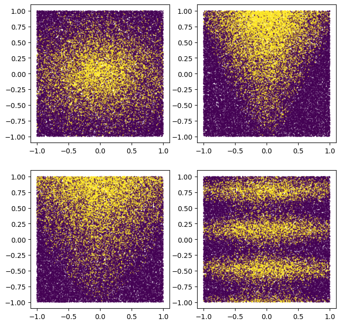
Note that this pattern is smooth and not axis aligned. This will advantage the neural network models. This is because it is easier for a neural network than for a decision tree to have round and non aligned decision boundaries.

On the other hand, we will train the model on a small datasets with 2500 examples. This will advantage the decision forest models. This is because decision forests are much more efficient, using all the available information from the examples (decision forests are "sample efficient").

Our ensemble of neural networks and decision forests will use the best of both worlds.

Let's create a train and test tf.data.Dataset:

def make_tf_dataset(batch_size=64, **args):
  features, labels = make_dataset(**args)
  return tf.data.Dataset.from_tensor_slices(
      (features, labels)).batch(batch_size)


num_features = 10

train_dataset = make_tf_dataset(
    num_examples=2500, num_features=num_features, batch_size=100, seed=1234)
test_dataset = make_tf_dataset(
    num_examples=10000, num_features=num_features, batch_size=100, seed=5678)

Model structure

Define the model structure as follows:

# Input features.
raw_features = tf_keras.layers.Input(shape=(num_features,))

# Stage 1
# =======

# Common learnable pre-processing
preprocessor = tf_keras.layers.Dense(10, activation=tf.nn.relu6)
preprocess_features = preprocessor(raw_features)

# Stage 2
# =======

# Model #1: NN
m1_z1 = tf_keras.layers.Dense(5, activation=tf.nn.relu6)(preprocess_features)
m1_pred = tf_keras.layers.Dense(1, activation=tf.nn.sigmoid)(m1_z1)

# Model #2: NN
m2_z1 = tf_keras.layers.Dense(5, activation=tf.nn.relu6)(preprocess_features)
m2_pred = tf_keras.layers.Dense(1, activation=tf.nn.sigmoid)(m2_z1)


# Model #3: DF
model_3 = tfdf.keras.RandomForestModel(num_trees=1000, random_seed=1234)
m3_pred = model_3(preprocess_features)

# Model #4: DF
model_4 = tfdf.keras.RandomForestModel(
    num_trees=1000,
    #split_axis="SPARSE_OBLIQUE", # Uncomment this line to increase the quality of this model
    random_seed=4567)
m4_pred = model_4(preprocess_features)

# Since TF-DF uses deterministic learning algorithms, you should set the model's
# training seed to different values otherwise both
# `tfdf.keras.RandomForestModel` will be exactly the same.

# Stage 3
# =======

mean_nn_only = tf.reduce_mean(tf.stack([m1_pred, m2_pred], axis=0), axis=0)
mean_nn_and_df = tf.reduce_mean(
    tf.stack([m1_pred, m2_pred, m3_pred, m4_pred], axis=0), axis=0)

# Keras Models
# ============

ensemble_nn_only = tf_keras.models.Model(raw_features, mean_nn_only)
ensemble_nn_and_df = tf_keras.models.Model(raw_features, mean_nn_and_df)

Warning: The `num_threads` constructor argument is not set and the number of CPU is os.cpu_count()=32 > 32. Setting num_threads to 32. Set num_threads manually to use more than 32 cpus.
WARNING:absl:The `num_threads` constructor argument is not set and the number of CPU is os.cpu_count()=32 > 32. Setting num_threads to 32. Set num_threads manually to use more than 32 cpus.
Use /tmpfs/tmp/tmp5rudwfpk as temporary training directory
Warning: The model was called directly (i.e. using `model(data)` instead of using `model.predict(data)`) before being trained. The model will only return zeros until trained. The output shape might change after training Tensor("inputs:0", shape=(None, 10), dtype=float32)
WARNING:absl:The model was called directly (i.e. using `model(data)` instead of using `model.predict(data)`) before being trained. The model will only return zeros until trained. The output shape might change after training Tensor("inputs:0", shape=(None, 10), dtype=float32)
Warning: The `num_threads` constructor argument is not set and the number of CPU is os.cpu_count()=32 > 32. Setting num_threads to 32. Set num_threads manually to use more than 32 cpus.
WARNING:absl:The `num_threads` constructor argument is not set and the number of CPU is os.cpu_count()=32 > 32. Setting num_threads to 32. Set num_threads manually to use more than 32 cpus.
Use /tmpfs/tmp/tmp7z3k5oog as temporary training directory
Warning: The model was called directly (i.e. using `model(data)` instead of using `model.predict(data)`) before being trained. The model will only return zeros until trained. The output shape might change after training Tensor("inputs:0", shape=(None, 10), dtype=float32)
WARNING:absl:The model was called directly (i.e. using `model(data)` instead of using `model.predict(data)`) before being trained. The model will only return zeros until trained. The output shape might change after training Tensor("inputs:0", shape=(None, 10), dtype=float32)

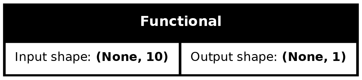
Before you train the model, you can plot it to check if it is similar to the initial diagram.

from keras.utils import plot_model

plot_model(ensemble_nn_and_df, to_file="/tmp/model.png", show_shapes=True)

png

Model training

First train the preprocessing and two neural network layers using the backpropagation algorithm.

%%time
ensemble_nn_only.compile(
        optimizer=tf_keras.optimizers.Adam(),
        loss=tf_keras.losses.BinaryCrossentropy(),
        metrics=["accuracy"])

ensemble_nn_only.fit(train_dataset, epochs=20, validation_data=test_dataset)

Epoch 1/20
WARNING: All log messages before absl::InitializeLog() is called are written to STDERR
I0000 00:00:1713611529.601020   11701 service.cc:145] XLA service 0x7f48904d48d0 initialized for platform CUDA (this does not guarantee that XLA will be used). Devices:
I0000 00:00:1713611529.601060   11701 service.cc:153]   StreamExecutor device (0): Tesla T4, Compute Capability 7.5
I0000 00:00:1713611529.601064   11701 service.cc:153]   StreamExecutor device (1): Tesla T4, Compute Capability 7.5
I0000 00:00:1713611529.601067   11701 service.cc:153]   StreamExecutor device (2): Tesla T4, Compute Capability 7.5
I0000 00:00:1713611529.601069   11701 service.cc:153]   StreamExecutor device (3): Tesla T4, Compute Capability 7.5
I0000 00:00:1713611529.771938   11701 device_compiler.h:188] Compiled cluster using XLA!  This line is logged at most once for the lifetime of the process.
25/25 [==============================] - 15s 33ms/step - loss: 0.5756 - accuracy: 0.7500 - val_loss: 0.5714 - val_accuracy: 0.7392
Epoch 2/20
25/25 [==============================] - 0s 11ms/step - loss: 0.5524 - accuracy: 0.7500 - val_loss: 0.5543 - val_accuracy: 0.7392
Epoch 3/20
25/25 [==============================] - 0s 10ms/step - loss: 0.5351 - accuracy: 0.7500 - val_loss: 0.5406 - val_accuracy: 0.7392
Epoch 4/20
25/25 [==============================] - 0s 10ms/step - loss: 0.5209 - accuracy: 0.7500 - val_loss: 0.5287 - val_accuracy: 0.7392
Epoch 5/20
25/25 [==============================] - 0s 10ms/step - loss: 0.5083 - accuracy: 0.7500 - val_loss: 0.5176 - val_accuracy: 0.7392
Epoch 6/20
25/25 [==============================] - 0s 10ms/step - loss: 0.4967 - accuracy: 0.7500 - val_loss: 0.5072 - val_accuracy: 0.7392
Epoch 7/20
25/25 [==============================] - 0s 10ms/step - loss: 0.4856 - accuracy: 0.7512 - val_loss: 0.4973 - val_accuracy: 0.7397
Epoch 8/20
25/25 [==============================] - 0s 10ms/step - loss: 0.4753 - accuracy: 0.7524 - val_loss: 0.4882 - val_accuracy: 0.7421
Epoch 9/20
25/25 [==============================] - 0s 10ms/step - loss: 0.4658 - accuracy: 0.7572 - val_loss: 0.4799 - val_accuracy: 0.7454
Epoch 10/20
25/25 [==============================] - 0s 10ms/step - loss: 0.4572 - accuracy: 0.7600 - val_loss: 0.4726 - val_accuracy: 0.7500
Epoch 11/20
25/25 [==============================] - 0s 10ms/step - loss: 0.4498 - accuracy: 0.7668 - val_loss: 0.4664 - val_accuracy: 0.7575
Epoch 12/20
25/25 [==============================] - 0s 10ms/step - loss: 0.4435 - accuracy: 0.7748 - val_loss: 0.4612 - val_accuracy: 0.7637
Epoch 13/20
25/25 [==============================] - 0s 11ms/step - loss: 0.4382 - accuracy: 0.7780 - val_loss: 0.4569 - val_accuracy: 0.7678
Epoch 14/20
25/25 [==============================] - 0s 10ms/step - loss: 0.4339 - accuracy: 0.7832 - val_loss: 0.4534 - val_accuracy: 0.7702
Epoch 15/20
25/25 [==============================] - 0s 11ms/step - loss: 0.4302 - accuracy: 0.7888 - val_loss: 0.4504 - val_accuracy: 0.7731
Epoch 16/20
25/25 [==============================] - 0s 10ms/step - loss: 0.4269 - accuracy: 0.7920 - val_loss: 0.4477 - val_accuracy: 0.7768
Epoch 17/20
25/25 [==============================] - 0s 10ms/step - loss: 0.4239 - accuracy: 0.7924 - val_loss: 0.4452 - val_accuracy: 0.7786
Epoch 18/20
25/25 [==============================] - 0s 10ms/step - loss: 0.4211 - accuracy: 0.7936 - val_loss: 0.4429 - val_accuracy: 0.7800
Epoch 19/20
25/25 [==============================] - 0s 10ms/step - loss: 0.4184 - accuracy: 0.7976 - val_loss: 0.4406 - val_accuracy: 0.7819
Epoch 20/20
25/25 [==============================] - 0s 10ms/step - loss: 0.4158 - accuracy: 0.7992 - val_loss: 0.4382 - val_accuracy: 0.7836
CPU times: user 20.7 s, sys: 1.36 s, total: 22 s
Wall time: 19.6 s
<tf_keras.src.callbacks.History at 0x7f4a4c0fa3a0>

Let's evaluate the preprocessing and the part with the two neural networks only:

evaluation_nn_only = ensemble_nn_only.evaluate(test_dataset, return_dict=True)
print("Accuracy (NN #1 and #2 only): ", evaluation_nn_only["accuracy"])
print("Loss (NN #1 and #2 only): ", evaluation_nn_only["loss"])

100/100 [==============================] - 0s 2ms/step - loss: 0.4382 - accuracy: 0.7836
Accuracy (NN #1 and #2 only):  0.7835999727249146
Loss (NN #1 and #2 only):  0.438231498003006

Let's train the two Decision Forest components (one after another).

%%time
train_dataset_with_preprocessing = train_dataset.map(lambda x,y: (preprocessor(x), y))
test_dataset_with_preprocessing = test_dataset.map(lambda x,y: (preprocessor(x), y))

model_3.fit(train_dataset_with_preprocessing)
model_4.fit(train_dataset_with_preprocessing)

WARNING:tensorflow:AutoGraph could not transform <function <lambda> at 0x7f4b7b5d91f0> and will run it as-is.
Cause: could not parse the source code of <function <lambda> at 0x7f4b7b5d91f0>: no matching AST found among candidates:

To silence this warning, decorate the function with @tf.autograph.experimental.do_not_convert
WARNING:tensorflow:AutoGraph could not transform <function <lambda> at 0x7f4b7b5d91f0> and will run it as-is.
Cause: could not parse the source code of <function <lambda> at 0x7f4b7b5d91f0>: no matching AST found among candidates:

To silence this warning, decorate the function with @tf.autograph.experimental.do_not_convert
WARNING: AutoGraph could not transform <function <lambda> at 0x7f4b7b5d91f0> and will run it as-is.
Cause: could not parse the source code of <function <lambda> at 0x7f4b7b5d91f0>: no matching AST found among candidates:

To silence this warning, decorate the function with @tf.autograph.experimental.do_not_convert
WARNING:tensorflow:AutoGraph could not transform <function <lambda> at 0x7f4b7ba3eee0> and will run it as-is.
Cause: could not parse the source code of <function <lambda> at 0x7f4b7ba3eee0>: no matching AST found among candidates:

To silence this warning, decorate the function with @tf.autograph.experimental.do_not_convert
WARNING:tensorflow:AutoGraph could not transform <function <lambda> at 0x7f4b7ba3eee0> and will run it as-is.
Cause: could not parse the source code of <function <lambda> at 0x7f4b7ba3eee0>: no matching AST found among candidates:

To silence this warning, decorate the function with @tf.autograph.experimental.do_not_convert
WARNING: AutoGraph could not transform <function <lambda> at 0x7f4b7ba3eee0> and will run it as-is.
Cause: could not parse the source code of <function <lambda> at 0x7f4b7ba3eee0>: no matching AST found among candidates:

To silence this warning, decorate the function with @tf.autograph.experimental.do_not_convert
Reading training dataset...
Training dataset read in 0:00:03.699343. Found 2500 examples.
Training model...
[INFO 24-04-20 11:12:20.9165 UTC kernel.cc:1233] Loading model from path /tmpfs/tmp/tmp5rudwfpk/model/ with prefix 3da3a8649d9e4cb4
Model trained in 0:00:02.061496
Compiling model...
[INFO 24-04-20 11:12:22.0091 UTC decision_forest.cc:734] Model loaded with 1000 root(s), 355690 node(s), and 10 input feature(s).
[INFO 24-04-20 11:12:22.0091 UTC abstract_model.cc:1344] Engine "RandomForestOptPred" built
[INFO 24-04-20 11:12:22.0091 UTC kernel.cc:1061] Use fast generic engine
Model compiled.
Reading training dataset...
Training dataset read in 0:00:00.231041. Found 2500 examples.
Training model...
[INFO 24-04-20 11:12:23.7301 UTC kernel.cc:1233] Loading model from path /tmpfs/tmp/tmp7z3k5oog/model/ with prefix 8b0da5e131c043b2
Model trained in 0:00:01.916593
Compiling model...
[INFO 24-04-20 11:12:24.7575 UTC decision_forest.cc:734] Model loaded with 1000 root(s), 357028 node(s), and 10 input feature(s).
[INFO 24-04-20 11:12:24.7576 UTC kernel.cc:1061] Use fast generic engine
Model compiled.
CPU times: user 22.9 s, sys: 1.73 s, total: 24.6 s
Wall time: 8.74 s
<tf_keras.src.callbacks.History at 0x7f4b7b6fcee0>

And let's evaluate the Decision Forests individually.

model_3.compile(["accuracy"])
model_4.compile(["accuracy"])

evaluation_df3_only = model_3.evaluate(
    test_dataset_with_preprocessing, return_dict=True)
evaluation_df4_only = model_4.evaluate(
    test_dataset_with_preprocessing, return_dict=True)

print("Accuracy (DF #3 only): ", evaluation_df3_only["accuracy"])
print("Accuracy (DF #4 only): ", evaluation_df4_only["accuracy"])

100/100 [==============================] - 2s 10ms/step - loss: 0.0000e+00 - accuracy: 0.7990
100/100 [==============================] - 1s 10ms/step - loss: 0.0000e+00 - accuracy: 0.7989
Accuracy (DF #3 only):  0.7990000247955322
Accuracy (DF #4 only):  0.7989000082015991

Let's evaluate the entire model composition:

ensemble_nn_and_df.compile(
    loss=tf_keras.losses.BinaryCrossentropy(), metrics=["accuracy"])

evaluation_nn_and_df = ensemble_nn_and_df.evaluate(
    test_dataset, return_dict=True)

print("Accuracy (2xNN and 2xDF): ", evaluation_nn_and_df["accuracy"])
print("Loss (2xNN and 2xDF): ", evaluation_nn_and_df["loss"])

100/100 [==============================] - 2s 10ms/step - loss: 0.4226 - accuracy: 0.7953
Accuracy (2xNN and 2xDF):  0.7953000068664551
Loss (2xNN and 2xDF):  0.4225609302520752

To finish, let's finetune the neural network layer a bit more. Note that we do not finetune the pre-trained embedding as the DF models depends on it (unless we would also retrain them after).

In summary, you have:

print(f"Accuracy (NN #1 and #2 only):\t{evaluation_nn_only['accuracy']:.6f}")
print(f"Accuracy (DF #3 only):\t\t{evaluation_df3_only['accuracy']:.6f}")
print(f"Accuracy (DF #4 only):\t\t{evaluation_df4_only['accuracy']:.6f}")
print("----------------------------------------")
print(f"Accuracy (2xNN and 2xDF):\t{evaluation_nn_and_df['accuracy']:.6f}")


def delta_percent(src_eval, key):
  src_acc = src_eval["accuracy"]
  final_acc = evaluation_nn_and_df["accuracy"]
  increase = final_acc - src_acc
  print(f"\t\t\t\t  {increase:+.6f} over {key}")


delta_percent(evaluation_nn_only, "NN #1 and #2 only")
delta_percent(evaluation_df3_only, "DF #3 only")
delta_percent(evaluation_df4_only, "DF #4 only")

Accuracy (NN #1 and #2 only): 0.783600
Accuracy (DF #3 only):        0.799000
Accuracy (DF #4 only):        0.798900
----------------------------------------
Accuracy (2xNN and 2xDF): 0.795300
                  +0.011700 over NN #1 and #2 only
                  -0.003700 over DF #3 only
                  -0.003600 over DF #4 only

Here, you can see that the composed model performs better than its individual parts. This is why ensembles work so well.

What's next?

In this example, you saw how to combine decision forests with neural networks. An extra step would be to further train the neural network and the decision forests together.

In addition, for the sake of clarity, the decision forests received only the preprocessed input. However, decision forests are generally great are consuming raw data. The model would be improved by also feeding the raw features to the decision forest models.

In this example, the final model is the average of the predictions of the individual models. This solution works well if all of the model perform more of less with the same. However, if one of the sub-models is very good, aggregating it with other models might actually be detrimental (or vice-versa; for example try to reduce the number of examples from 1k and see how it hurts the neural networks a lot; or enable the SPARSE_OBLIQUE split in the second Random Forest model).

Composing Decision Forest and Neural Network models Stay organized with collections Save and categorize content based on your preferences.