
|
|
|
 View on GitHub View on GitHub
|
|
Introduction
Leo Breiman, the author of the random forest learning algorithm, proposed a method to measure the proximity (also known as similarity) between two examples using a pre-trained Random Forest (RF) model. He qualifies this method as "[...] one of the most useful tools in random forests.". In this Notebook, we implement this method and show how to use it to interpret models.
This notebook is implemented using the TensorFlow Decision Forests library. This document is easier to understand if you are familiar with the content of the Beginner colab.
Proximities
A proximity (or a similarity) between two examples is a number indicating how "close" those two examples are. Following is an example of similarity in between the 3 examples \(\{e_1, e_2, e_3\}\):
\[ \mathrm{proxy}(e_1, e_2) = 0.1 \\ \mathrm{proxy}(e_2, e_3) = 9.6 \\ \mathrm{proxy}(e_3, e_1) = 4.1 \\ \]
For convenience, the proximity between examples is represented in matrix form:
| \(e_1\) | \(e_2\) | \(e_3\) | |
|---|---|---|---|
| \(e_1\) | \(\mathrm{proxy}(e_1, e_1)\) | \(\mathrm{proxy}(e_1, e_2)\) | \(\mathrm{proxy}(e_1, e_3)\) |
| \(e_2\) | \(\mathrm{proxy}(e_2, e_1)\) | \(\mathrm{proxy}(e_2, e_2)\) | \(\mathrm{proxy}(e_2, e_3)\) |
| \(e_3\) | \(\mathrm{proxy}(e_3, e_1)\) | \(\mathrm{proxy}(e_3, e_2)\) | \(\mathrm{proxy}(e_3, e_3)\) |
Proximities are used in multiple data analysis techniques, including clustering, dimensionality reductions or nearest neighbor analysis. For this reason, it is a great tool for models and predictions interpretation.
Unfortunately, measuring the proximity between two tabular examples is not straightforward as different columns might describe different quantities. For example, try to define the proximity in between the following examples.
| species | weight | num_legs | age | sex |
|---|---|---|---|---|
| cat | 2 kg | 4 | 2 y | male |
| dog | 6 kg | 4 | 12 y | female |
| spider | 5 g | 8 | 3 weeks | female |
To define the similarity between two rows in the table above, you need to specify how much a difference in weight compares to a difference in the number of legs, or in ages. In addition, relations might be non-linear or be conditional on other columns. For example, dogs live longer than spiders, so maybe, a one year difference for a spider should not count the same one year of age for a dog.
Instead of manually defining those relations, Breiman's proximity turns a random forest model (which we know how to train on a tabular dataset), into a proximity metric.
Proximities with random forests
A random forest is a collection of decision trees. The prediction of the random the aggregation of the predictions of the individual trees. The prediction of a decision tree is computed by routing an example from the root to forest is one of the leaves according to node conditions. The leaf reached by the example \(i\) in the tree \(t\) is called its active leaf and noted \(\mathrm{leaf}(i,t)\)
Breiman defines the proximity between two examples as the ratio of shared active leafs between those two examples. Formally, the proximity between example \(i\) and example \(j\) is:
\[ \mathrm{prox}(i,j) = \mathrm{prox}(j,i) = \frac{1}{|\mathrm{Trees}|} \sum_{t \in \mathrm{Trees} } \left[ \mathrm{leaf}(i,t) = \mathrm{leaf}(j,t) \right] \]
with \(\mathrm{leaf}(j,t)\) the index of the active leaf for the example \(j\) in the tree \(t\).
Informally, if two examples are often routed to the same leaves (i.e. the two examples have the same active leaves), those examples are similar.
Let's implement this proximity function and use it in some examples.
Setup
# Install TensorFlow Dececision Forests and the dependencies used in this colab.pip install tensorflow_decision_forests plotly scikit-learn wurlitzer -U -qq
import tensorflow_decision_forests as tfdf

import matplotlib.colors as mcolors
import math
import os
import numpy as np
import pandas as pd
from sklearn.manifold import TSNE
import matplotlib.pyplot as plt
from plotly.offline import iplot
import plotly.graph_objs as go
2026-01-12 15:08:34.826005: E external/local_xla/xla/stream_executor/cuda/cuda_fft.cc:467] Unable to register cuFFT factory: Attempting to register factory for plugin cuFFT when one has already been registered
WARNING: All log messages before absl::InitializeLog() is called are written to STDERR
E0000 00:00:1768230514.848493  185546 cuda_dnn.cc:8579] Unable to register cuDNN factory: Attempting to register factory for plugin cuDNN when one has already been registered
E0000 00:00:1768230514.856110  185546 cuda_blas.cc:1407] Unable to register cuBLAS factory: Attempting to register factory for plugin cuBLAS when one has already been registered
W0000 00:00:1768230514.874478  185546 computation_placer.cc:177] computation placer already registered. Please check linkage and avoid linking the same target more than once.
W0000 00:00:1768230514.874496  185546 computation_placer.cc:177] computation placer already registered. Please check linkage and avoid linking the same target more than once.
W0000 00:00:1768230514.874499  185546 computation_placer.cc:177] computation placer already registered. Please check linkage and avoid linking the same target more than once.
W0000 00:00:1768230514.874501  185546 computation_placer.cc:177] computation placer already registered. Please check linkage and avoid linking the same target more than once.
Train a Random Forest model
The method relies on a pre-trained random forest model. First, we train a random forest model with TensorFlow Decision Forests library on the Adult binary classification dataset. The Adult dataset is well suited for this example as it contains columns that don't have a natural way to be compared.
# Download a copy of the adult dataset.wget -q https://raw.githubusercontent.com/google/yggdrasil-decision-forests/main/yggdrasil_decision_forests/test_data/dataset/adult_train.csv -O /tmp/adult_train.csvwget -q https://raw.githubusercontent.com/google/yggdrasil-decision-forests/main/yggdrasil_decision_forests/test_data/dataset/adult_test.csv -O /tmp/adult_test.csv
# Load the dataset in memory
train_df = pd.read_csv("/tmp/adult_train.csv")
test_df = pd.read_csv("/tmp/adult_test.csv")

# , and convert it into a TensorFlow dataset.
train_ds = tfdf.keras.pd_dataframe_to_tf_dataset(train_df, label="income")
test_ds = tfdf.keras.pd_dataframe_to_tf_dataset(test_df, label="income")
I0000 00:00:1768230520.696209  185546 gpu_device.cc:2019] Created device /job:localhost/replica:0/task:0/device:GPU:0 with 13638 MB memory:  -> device: 0, name: Tesla T4, pci bus id: 0000:00:05.0, compute capability: 7.5
I0000 00:00:1768230520.698415  185546 gpu_device.cc:2019] Created device /job:localhost/replica:0/task:0/device:GPU:1 with 13756 MB memory:  -> device: 1, name: Tesla T4, pci bus id: 0000:00:06.0, compute capability: 7.5
I0000 00:00:1768230520.700853  185546 gpu_device.cc:2019] Created device /job:localhost/replica:0/task:0/device:GPU:2 with 13756 MB memory:  -> device: 2, name: Tesla T4, pci bus id: 0000:00:07.0, compute capability: 7.5
I0000 00:00:1768230520.703137  185546 gpu_device.cc:2019] Created device /job:localhost/replica:0/task:0/device:GPU:3 with 13756 MB memory:  -> device: 3, name: Tesla T4, pci bus id: 0000:00:08.0, compute capability: 7.5
Following are the first five examples of the training dataset. Notice that different columns represent different quantities. For example, how would you compare the distance between relationship and age?
# Print the first 5 examples.
train_df.head()
A Random Forest is trained as follows:
# Train a Random Forest
model = tfdf.keras.RandomForestModel(num_trees=1000)
model.fit(train_ds)
Warning: The `num_threads` constructor argument is not set and the number of CPU is os.cpu_count()=32 > 32. Setting num_threads to 32. Set num_threads manually to use more than 32 cpus.
WARNING:absl:The `num_threads` constructor argument is not set and the number of CPU is os.cpu_count()=32 > 32. Setting num_threads to 32. Set num_threads manually to use more than 32 cpus.
Use /tmpfs/tmp/tmpuevt5z8y as temporary training directory
Reading training dataset...
Training dataset read in 0:00:03.919743. Found 22792 examples.
Training model...
WARNING: All log messages before absl::InitializeLog() is called are written to STDERR
I0000 00:00:1768230525.068555  185546 kernel.cc:782] Start Yggdrasil model training
I0000 00:00:1768230525.068605  185546 kernel.cc:783] Collect training examples
I0000 00:00:1768230525.068612  185546 kernel.cc:795] Dataspec guide:
column_guides {
  column_name_pattern: "^__LABEL$"
  type: CATEGORICAL
  categorial {
    min_vocab_frequency: 0
    max_vocab_count: -1
  }
}
default_column_guide {
  categorial {
    max_vocab_count: 2000
  }
  discretized_numerical {
    maximum_num_bins: 255
  }
}
ignore_columns_without_guides: false
detect_numerical_as_discretized_numerical: false

I0000 00:00:1768230525.068970  185546 kernel.cc:401] Number of batches: 23
I0000 00:00:1768230525.068983  185546 kernel.cc:402] Number of examples: 22792
I0000 00:00:1768230525.075569  185546 data_spec_inference.cc:354] 1 item(s) have been pruned (i.e. they are considered out of dictionary) for the column native_country (40 item(s) left) because min_value_count=5 and max_number_of_unique_values=2000
I0000 00:00:1768230525.075599  185546 data_spec_inference.cc:354] 1 item(s) have been pruned (i.e. they are considered out of dictionary) for the column occupation (13 item(s) left) because min_value_count=5 and max_number_of_unique_values=2000
I0000 00:00:1768230525.075616  185546 data_spec_inference.cc:354] 1 item(s) have been pruned (i.e. they are considered out of dictionary) for the column workclass (7 item(s) left) because min_value_count=5 and max_number_of_unique_values=2000
I0000 00:00:1768230525.081517  185546 kernel.cc:802] Training dataset:
Number of records: 22792
Number of columns: 15

Number of columns by type:
    CATEGORICAL: 9 (60%)
    NUMERICAL: 6 (40%)

Columns:

CATEGORICAL: 9 (60%)
    0: "__LABEL" CATEGORICAL integerized vocab-size:3 no-ood-item
    4: "education" CATEGORICAL has-dict vocab-size:17 zero-ood-items most-frequent:"HS-grad" 7340 (32.2043%)
    8: "marital_status" CATEGORICAL has-dict vocab-size:8 zero-ood-items most-frequent:"Married-civ-spouse" 10431 (45.7661%)
    9: "native_country" CATEGORICAL num-nas:407 (1.78571%) has-dict vocab-size:41 num-oods:1 (0.00446728%) most-frequent:"United-States" 20436 (91.2933%)
    10: "occupation" CATEGORICAL num-nas:1260 (5.52826%) has-dict vocab-size:14 num-oods:4 (0.018577%) most-frequent:"Prof-specialty" 2870 (13.329%)
    11: "race" CATEGORICAL has-dict vocab-size:6 zero-ood-items most-frequent:"White" 19467 (85.4115%)
    12: "relationship" CATEGORICAL has-dict vocab-size:7 zero-ood-items most-frequent:"Husband" 9191 (40.3256%)
    13: "sex" CATEGORICAL has-dict vocab-size:3 zero-ood-items most-frequent:"Male" 15165 (66.5365%)
    14: "workclass" CATEGORICAL num-nas:1257 (5.51509%) has-dict vocab-size:8 num-oods:3 (0.0139308%) most-frequent:"Private" 15879 (73.7358%)

NUMERICAL: 6 (40%)
    1: "age" NUMERICAL mean:38.6153 min:17 max:90 sd:13.661
    2: "capital_gain" NUMERICAL mean:1081.9 min:0 max:99999 sd:7509.48
    3: "capital_loss" NUMERICAL mean:87.2806 min:0 max:4356 sd:403.01
    5: "education_num" NUMERICAL mean:10.0927 min:1 max:16 sd:2.56427
    6: "fnlwgt" NUMERICAL mean:189879 min:12285 max:1.4847e+06 sd:106423
    7: "hours_per_week" NUMERICAL mean:40.3955 min:1 max:99 sd:12.249

Terminology:
    nas: Number of non-available (i.e. missing) values.
    ood: Out of dictionary.
    manually-defined: Attribute whose type is manually defined by the user, i.e., the type was not automatically inferred.
    tokenized: The attribute value is obtained through tokenization.
    has-dict: The attribute is attached to a string dictionary e.g. a categorical attribute stored as a string.
    vocab-size: Number of unique values.

I0000 00:00:1768230525.081566  185546 kernel.cc:818] Configure learner
I0000 00:00:1768230525.081783  185546 kernel.cc:831] Training config:
learner: "RANDOM_FOREST"
features: "^age$"
features: "^capital_gain$"
features: "^capital_loss$"
features: "^education$"
features: "^education_num$"
features: "^fnlwgt$"
features: "^hours_per_week$"
features: "^marital_status$"
features: "^native_country$"
features: "^occupation$"
features: "^race$"
features: "^relationship$"
features: "^sex$"
features: "^workclass$"
label: "^__LABEL$"
task: CLASSIFICATION
random_seed: 123456
metadata {
  framework: "TF Keras"
}
pure_serving_model: false
[yggdrasil_decision_forests.model.random_forest.proto.random_forest_config] {
  num_trees: 1000
  decision_tree {
    max_depth: 16
    min_examples: 5
    in_split_min_examples_check: true
    keep_non_leaf_label_distribution: true
    num_candidate_attributes: 0
    missing_value_policy: GLOBAL_IMPUTATION
    allow_na_conditions: false
    categorical_set_greedy_forward {
      sampling: 0.1
      max_num_items: -1
      min_item_frequency: 1
    }
    growing_strategy_local {
    }
    categorical {
      cart {
      }
    }
    axis_aligned_split {
    }
    internal {
      sorting_strategy: PRESORTED
    }
    uplift {
      min_examples_in_treatment: 5
      split_score: KULLBACK_LEIBLER
    }
    numerical_vector_sequence {
      max_num_test_examples: 1000
      num_random_selected_anchors: 100
    }
  }
  winner_take_all_inference: true
  compute_oob_performances: true
  compute_oob_variable_importances: false
  num_oob_variable_importances_permutations: 1
  bootstrap_training_dataset: true
  bootstrap_size_ratio: 1
  adapt_bootstrap_size_ratio_for_maximum_training_duration: false
  sampling_with_replacement: true
}

I0000 00:00:1768230525.082155  185546 kernel.cc:834] Deployment config:
cache_path: "/tmpfs/tmp/tmpuevt5z8y/working_cache"
num_threads: 32
try_resume_training: true

I0000 00:00:1768230525.082355  185768 kernel.cc:895] Train model
I0000 00:00:1768230525.082517  185768 random_forest.cc:438] Training random forest on 22792 example(s) and 14 feature(s).
I0000 00:00:1768230525.089757  185768 gpu.cc:93] Cannot initialize GPU: Not compiled with GPU support
I0000 00:00:1768230525.151600  185791 random_forest.cc:865] Train tree 1/1000 accuracy:0.83445 logloss:5.96701 [index:8 total:0.06s tree:0.06s]
I0000 00:00:1768230525.191818  185813 random_forest.cc:865] Train tree 11/1000 accuracy:0.856695 logloss:2.8676 [index:27 total:0.10s tree:0.10s]
I0000 00:00:1768230525.229763  185803 random_forest.cc:865] Train tree 21/1000 accuracy:0.859951 logloss:1.97867 [index:18 total:0.14s tree:0.14s]
I0000 00:00:1768230525.270777  185812 random_forest.cc:865] Train tree 31/1000 accuracy:0.862276 logloss:1.58216 [index:26 total:0.18s tree:0.18s]
I0000 00:00:1768230525.311815  185793 random_forest.cc:865] Train tree 41/1000 accuracy:0.862101 logloss:1.34302 [index:38 total:0.22s tree:0.14s]
I0000 00:00:1768230525.350905  185806 random_forest.cc:865] Train tree 51/1000 accuracy:0.862057 logloss:1.21212 [index:49 total:0.26s tree:0.13s]
I0000 00:00:1768230525.390341  185797 random_forest.cc:865] Train tree 61/1000 accuracy:0.86311 logloss:1.12156 [index:58 total:0.30s tree:0.14s]
I0000 00:00:1768230525.430094  185789 random_forest.cc:865] Train tree 71/1000 accuracy:0.863461 logloss:1.02083 [index:71 total:0.34s tree:0.13s]
I0000 00:00:1768230525.466551  185811 random_forest.cc:865] Train tree 81/1000 accuracy:0.863812 logloss:0.96177 [index:80 total:0.38s tree:0.12s]
I0000 00:00:1768230525.505402  185798 random_forest.cc:865] Train tree 91/1000 accuracy:0.864294 logloss:0.918772 [index:91 total:0.41s tree:0.12s]
I0000 00:00:1768230525.528704  185795 random_forest.cc:865] Train tree 120/1000 accuracy:0.8639 logloss:0.891848 [index:118 total:0.44s tree:0.04s]
I0000 00:00:1768230525.647896  185810 random_forest.cc:865] Train tree 130/1000 accuracy:0.864163 logloss:0.775813 [index:129 total:0.56s tree:0.12s]
I0000 00:00:1768230525.686897  185794 random_forest.cc:865] Train tree 140/1000 accuracy:0.864031 logloss:0.746119 [index:140 total:0.60s tree:0.12s]
I0000 00:00:1768230525.724402  185788 random_forest.cc:865] Train tree 150/1000 accuracy:0.864075 logloss:0.71837 [index:148 total:0.63s tree:0.13s]
I0000 00:00:1768230525.763674  185804 random_forest.cc:865] Train tree 160/1000 accuracy:0.864338 logloss:0.709851 [index:157 total:0.67s tree:0.13s]
I0000 00:00:1768230525.803246  185785 random_forest.cc:865] Train tree 170/1000 accuracy:0.864689 logloss:0.68861 [index:166 total:0.71s tree:0.13s]
I0000 00:00:1768230525.816646  185807 random_forest.cc:865] Train tree 194/1000 accuracy:0.864777 logloss:0.678833 [index:193 total:0.73s tree:0.05s]
I0000 00:00:1768230525.934269  185785 random_forest.cc:865] Train tree 204/1000 accuracy:0.864996 logloss:0.638392 [index:201 total:0.84s tree:0.13s]
I0000 00:00:1768230525.969797  185802 random_forest.cc:865] Train tree 214/1000 accuracy:0.864996 logloss:0.624507 [index:214 total:0.88s tree:0.12s]
I0000 00:00:1768230526.010132  185797 random_forest.cc:865] Train tree 224/1000 accuracy:0.86504 logloss:0.62019 [index:222 total:0.92s tree:0.13s]
I0000 00:00:1768230526.048649  185789 random_forest.cc:865] Train tree 234/1000 accuracy:0.865216 logloss:0.614164 [index:232 total:0.96s tree:0.13s]
I0000 00:00:1768230526.086273  185786 random_forest.cc:865] Train tree 244/1000 accuracy:0.865348 logloss:0.603218 [index:244 total:0.99s tree:0.12s]
I0000 00:00:1768230526.123756  185812 random_forest.cc:865] Train tree 254/1000 accuracy:0.865304 logloss:0.600413 [index:251 total:1.03s tree:0.13s]
I0000 00:00:1768230526.163032  185801 random_forest.cc:865] Train tree 264/1000 accuracy:0.865216 logloss:0.595068 [index:262 total:1.07s tree:0.13s]
I0000 00:00:1768230526.177691  185797 random_forest.cc:865] Train tree 291/1000 accuracy:0.865304 logloss:0.595349 [index:288 total:1.09s tree:0.04s]
I0000 00:00:1768230526.297063  185792 random_forest.cc:865] Train tree 301/1000 accuracy:0.865435 logloss:0.57584 [index:300 total:1.21s tree:0.12s]
I0000 00:00:1768230526.333600  185784 random_forest.cc:865] Train tree 311/1000 accuracy:0.865435 logloss:0.568895 [index:310 total:1.24s tree:0.12s]
I0000 00:00:1768230526.364497  185784 random_forest.cc:865] Train tree 343/1000 accuracy:0.865216 logloss:0.567393 [index:342 total:1.27s tree:0.03s]
I0000 00:00:1768230526.477899  185798 random_forest.cc:865] Train tree 373/1000 accuracy:0.865084 logloss:0.546581 [index:373 total:1.39s tree:0.03s]
I0000 00:00:1768230526.598414  185787 random_forest.cc:865] Train tree 383/1000 accuracy:0.865348 logloss:0.539292 [index:382 total:1.51s tree:0.12s]
I0000 00:00:1768230526.635175  185792 random_forest.cc:865] Train tree 393/1000 accuracy:0.865786 logloss:0.538173 [index:393 total:1.54s tree:0.11s]
I0000 00:00:1768230526.656720  185784 random_forest.cc:865] Train tree 420/1000 accuracy:0.865523 logloss:0.534094 [index:417 total:1.57s tree:0.05s]
I0000 00:00:1768230526.778996  185784 random_forest.cc:865] Train tree 430/1000 accuracy:0.865567 logloss:0.523191 [index:429 total:1.69s tree:0.12s]
I0000 00:00:1768230526.817244  185803 random_forest.cc:865] Train tree 440/1000 accuracy:0.865304 logloss:0.52329 [index:440 total:1.73s tree:0.12s]
I0000 00:00:1768230526.854936  185790 random_forest.cc:865] Train tree 450/1000 accuracy:0.865348 logloss:0.522959 [index:449 total:1.76s tree:0.12s]
I0000 00:00:1768230526.891732  185812 random_forest.cc:865] Train tree 460/1000 accuracy:0.865084 logloss:0.519008 [index:460 total:1.80s tree:0.12s]
I0000 00:00:1768230526.931922  185802 random_forest.cc:865] Train tree 470/1000 accuracy:0.865348 logloss:0.518726 [index:469 total:1.84s tree:0.12s]
I0000 00:00:1768230526.968974  185788 random_forest.cc:865] Train tree 480/1000 accuracy:0.865655 logloss:0.518826 [index:479 total:1.88s tree:0.12s]
I0000 00:00:1768230527.006533  185807 random_forest.cc:865] Train tree 490/1000 accuracy:0.865304 logloss:0.517573 [index:490 total:1.92s tree:0.12s]
I0000 00:00:1768230527.044422  185797 random_forest.cc:865] Train tree 500/1000 accuracy:0.865348 logloss:0.512058 [index:498 total:1.95s tree:0.13s]
I0000 00:00:1768230527.082693  185806 random_forest.cc:865] Train tree 510/1000 accuracy:0.865567 logloss:0.509274 [index:507 total:1.99s tree:0.13s]
I0000 00:00:1768230527.119166  185796 random_forest.cc:865] Train tree 520/1000 accuracy:0.865611 logloss:0.506705 [index:518 total:2.03s tree:0.13s]
I0000 00:00:1768230527.156795  185801 random_forest.cc:865] Train tree 552/1000 accuracy:0.865391 logloss:0.506607 [index:552 total:2.07s tree:0.03s]
I0000 00:00:1768230527.212848  185797 random_forest.cc:865] Train tree 565/1000 accuracy:0.865523 logloss:0.502573 [index:564 total:2.12s tree:0.05s]
I0000 00:00:1768230527.321128  185791 random_forest.cc:865] Train tree 575/1000 accuracy:0.865391 logloss:0.48789 [index:574 total:2.23s tree:0.12s]
I0000 00:00:1768230527.333362  185811 random_forest.cc:865] Train tree 601/1000 accuracy:0.86526 logloss:0.487765 [index:599 total:2.24s tree:0.04s]
I0000 00:00:1768230527.451183  185805 random_forest.cc:865] Train tree 611/1000 accuracy:0.865567 logloss:0.4814 [index:610 total:2.36s tree:0.11s]
I0000 00:00:1768230527.488060  185796 random_forest.cc:865] Train tree 621/1000 accuracy:0.865523 logloss:0.478758 [index:618 total:2.40s tree:0.12s]
I0000 00:00:1768230527.528228  185810 random_forest.cc:865] Train tree 631/1000 accuracy:0.865172 logloss:0.477365 [index:628 total:2.44s tree:0.13s]
I0000 00:00:1768230527.565613  185797 random_forest.cc:865] Train tree 641/1000 accuracy:0.865084 logloss:0.475539 [index:640 total:2.47s tree:0.12s]
I0000 00:00:1768230527.603057  185785 random_forest.cc:865] Train tree 651/1000 accuracy:0.86526 logloss:0.475511 [index:650 total:2.51s tree:0.12s]
I0000 00:00:1768230527.633176  185812 random_forest.cc:865] Train tree 682/1000 accuracy:0.865391 logloss:0.475588 [index:681 total:2.54s tree:0.04s]
I0000 00:00:1768230527.756949  185793 random_forest.cc:865] Train tree 692/1000 accuracy:0.865216 logloss:0.4617 [index:693 total:2.67s tree:0.11s]
I0000 00:00:1768230527.791702  185793 random_forest.cc:865] Train tree 723/1000 accuracy:0.865084 logloss:0.461704 [index:723 total:2.70s tree:0.03s]
I0000 00:00:1768230527.907350  185793 random_forest.cc:865] Train tree 733/1000 accuracy:0.865611 logloss:0.449605 [index:732 total:2.82s tree:0.12s]
I0000 00:00:1768230527.947022  185811 random_forest.cc:865] Train tree 743/1000 accuracy:0.865435 logloss:0.448261 [index:739 total:2.86s tree:0.13s]
I0000 00:00:1768230527.986856  185785 random_forest.cc:865] Train tree 753/1000 accuracy:0.865216 logloss:0.445731 [index:749 total:2.90s tree:0.14s]
I0000 00:00:1768230528.027592  185810 random_forest.cc:865] Train tree 763/1000 accuracy:0.865391 logloss:0.444427 [index:761 total:2.94s tree:0.13s]
I0000 00:00:1768230528.037298  185784 random_forest.cc:865] Train tree 788/1000 accuracy:0.865479 logloss:0.443109 [index:788 total:2.95s tree:0.03s]
I0000 00:00:1768230528.163658  185791 random_forest.cc:865] Train tree 798/1000 accuracy:0.865348 logloss:0.44191 [index:797 total:3.07s tree:0.12s]
I0000 00:00:1768230528.200330  185800 random_forest.cc:865] Train tree 808/1000 accuracy:0.865391 logloss:0.440469 [index:806 total:3.11s tree:0.13s]
I0000 00:00:1768230528.212771  185792 random_forest.cc:865] Train tree 834/1000 accuracy:0.865479 logloss:0.440484 [index:833 total:3.12s tree:0.04s]
I0000 00:00:1768230528.338057  185799 random_forest.cc:865] Train tree 844/1000 accuracy:0.865435 logloss:0.43374 [index:843 total:3.25s tree:0.12s]
I0000 00:00:1768230528.377090  185785 random_forest.cc:865] Train tree 854/1000 accuracy:0.865172 logloss:0.432352 [index:850 total:3.29s tree:0.13s]
I0000 00:00:1768230528.414440  185805 random_forest.cc:865] Train tree 864/1000 accuracy:0.865348 logloss:0.432233 [index:864 total:3.32s tree:0.12s]
I0000 00:00:1768230528.454053  185792 random_forest.cc:865] Train tree 874/1000 accuracy:0.865523 logloss:0.432307 [index:874 total:3.36s tree:0.12s]
I0000 00:00:1768230528.477140  185783 random_forest.cc:865] Train tree 903/1000 accuracy:0.865567 logloss:0.430959 [index:902 total:3.39s tree:0.04s]
I0000 00:00:1768230528.600142  185798 random_forest.cc:865] Train tree 913/1000 accuracy:0.86526 logloss:0.431226 [index:913 total:3.51s tree:0.12s]
I0000 00:00:1768230528.637471  185793 random_forest.cc:865] Train tree 923/1000 accuracy:0.865216 logloss:0.431351 [index:920 total:3.55s tree:0.13s]
I0000 00:00:1768230528.642427  185788 random_forest.cc:865] Train tree 947/1000 accuracy:0.865172 logloss:0.431358 [index:946 total:3.55s tree:0.03s]
I0000 00:00:1768230528.734265  185796 random_forest.cc:865] Train tree 972/1000 accuracy:0.86526 logloss:0.428732 [index:971 total:3.64s tree:0.03s]
I0000 00:00:1768230528.854972  185796 random_forest.cc:865] Train tree 982/1000 accuracy:0.865216 logloss:0.424836 [index:980 total:3.76s tree:0.12s]
I0000 00:00:1768230528.894009  185802 random_forest.cc:865] Train tree 992/1000 accuracy:0.865172 logloss:0.423626 [index:990 total:3.80s tree:0.12s]
I0000 00:00:1768230528.922525  185810 random_forest.cc:865] Train tree 1000/1000 accuracy:0.865348 logloss:0.423661 [index:998 total:3.83s tree:0.12s]
I0000 00:00:1768230528.922790  185768 random_forest.cc:949] Final OOB metrics: accuracy:0.865348 logloss:0.423661
I0000 00:00:1768230529.552920  185768 kernel.cc:926] Export model in log directory: /tmpfs/tmp/tmpuevt5z8y with prefix ea44b85a04ab4298
I0000 00:00:1768230530.423948  185768 kernel.cc:944] Save model in resources
I0000 00:00:1768230530.427993  185546 abstract_model.cc:921] Model self evaluation:
Number of predictions (without weights): 22792
Number of predictions (with weights): 22792
Task: CLASSIFICATION
Label: __LABEL

Accuracy: 0.865348  CI95[W][0.861572 0.869054]
LogLoss: : 0.423661
ErrorRate: : 0.134652

Default Accuracy: : 0.759389
Default LogLoss: : 0.551783
Default ErrorRate: : 0.240611

Confusion Table:
truth\prediction
       1     2
1  16328   980
2   2089  3395
Total: 22792


WARNING: All log messages before absl::InitializeLog() is called are written to STDERR
I0000 00:00:1768230535.098393  185546 decision_forest.cc:808] Model loaded with 1000 root(s), 1262362 node(s), and 14 input feature(s).
I0000 00:00:1768230535.101653  185546 abstract_model.cc:1439] Engine "RandomForestGeneric" built
Model trained in 0:00:10.465669
Compiling model...
Model compiled.
<tf_keras.src.callbacks.History at 0x7ff8744da760>
The performance of the Random Forest model is:
model_inspector = model.make_inspector()
out_of_bag_accuracy = model_inspector.evaluation().accuracy
print(f"Out-of-bag accuracy: {out_of_bag_accuracy:.4f}")
Out-of-bag accuracy: 0.8653
This is an expected accuracy value for Random Forest models on this dataset. It indicates that the model is correctly trained.
We can also measure the accuracy of the model on the test datasets:
# The test accuracy is measured on the test datasets.
model.compile(["accuracy"])
test_accuracy = model.evaluate(test_ds, return_dict=True, verbose=0)["accuracy"]
print(f"Test accuracy: {test_accuracy:.4f}")
Test accuracy: 0.8663
Proximities
First, we inspect the number of trees in the model and the number of examples in the test datasets.
print("The model contains", model_inspector.num_trees(), "trees.")
print("The test dataset contains", test_df.shape[0], "examples.")
The model contains 1000 trees.
The test dataset contains 9769 examples.
The method predict_get_leaves() returns the index of the active leaf for each example and each tree.
leaves = model.predict_get_leaves(test_ds)
print("The leaf indices:\n", leaves)
WARNING:tensorflow:AutoGraph could not transform <function simple_ml_inference_leaf_index_op_with_handle at 0x7ff7855fbdc0> and will run it as-is.
Please report this to the TensorFlow team. When filing the bug, set the verbosity to 10 (on Linux, `export AUTOGRAPH_VERBOSITY=10`) and attach the full output.
Cause: could not get source code
To silence this warning, decorate the function with @tf.autograph.experimental.do_not_convert
WARNING: AutoGraph could not transform <function simple_ml_inference_leaf_index_op_with_handle at 0x7ff7855fbdc0> and will run it as-is.
Please report this to the TensorFlow team. When filing the bug, set the verbosity to 10 (on Linux, `export AUTOGRAPH_VERBOSITY=10`) and attach the full output.
Cause: could not get source code
To silence this warning, decorate the function with @tf.autograph.experimental.do_not_convert
The leaf indices:
 [[498 193 142 ... 457 221 198]
 [399 466 423 ... 288 420 444]
 [639 651 562 ... 608 636 625]
 ...
 [149 296 258 ... 153 310 316]
 [481 186 131 ... 432 192 153]
 [  9   0  28 ...   4   1  42]]
print("The predicted leaves have shape", leaves.shape,
      "(we expect [num_examples, num_trees]")
The predicted leaves have shape (9769, 1000) (we expect [num_examples, num_trees]
Here, leaves[i,j] is the index of the active leaf of the i-th
example in the j-th tree.
Next, we implement the \(\mathrm{prox}\) equation define earlier.
def compute_proximity(leaves, step_size=100):
  """Computes the proximity between each pair of examples.

  Args:
    leaves: A matrix of shape [num_example, num_tree] where the value [i,j] is
      the index of the leaf reached by example "i" in the tree "j".
    step_size: Size of the block of examples for the computation of the
      proximity. Does not impact the results.

  Returns:
    The example pair-wise proximity matrix of shape [n,n] with "n" the number of
    examples.
  """

  example_idx = 0
  num_examples = leaves.shape[0]
  t_leaves = np.transpose(leaves)
  proximities = []

  # Instead of computing the proximity in between all the examples at the same
  # time, we compute the similarity in blocks of "step_size" examples. This
  # makes the code more efficient with the the numpy broadcast.
  while example_idx < num_examples:
    end_idx = min(example_idx + step_size, num_examples)
    proximities.append(
        np.mean(
            leaves[..., np.newaxis] == t_leaves[:,
                                                example_idx:end_idx][np.newaxis,
                                                                     ...],
            axis=1))
    example_idx = end_idx
  return np.concatenate(proximities, axis=1)


proximity = compute_proximity(leaves)
print("The shape of proximity is", proximity.shape)
The shape of proximity is (9769, 9769)
Here, proximity[i,j] is the proximity in between the example i and j.
The proximity matrix:
proximity
array([[1.   , 0.   , 0.   , ..., 0.   , 0.053, 0.   ],
       [0.   , 1.   , 0.   , ..., 0.002, 0.   , 0.   ],
       [0.   , 0.   , 1.   , ..., 0.   , 0.   , 0.   ],
       ...,
       [0.   , 0.002, 0.   , ..., 1.   , 0.   , 0.   ],
       [0.053, 0.   , 0.   , ..., 0.   , 1.   , 0.   ],
       [0.   , 0.   , 0.   , ..., 0.   , 0.   , 1.   ]])
The proximity matrix has several interesting properties, notably, it is symmetrical, positive, and the diagonal elements are all 1.
Projection
Our first use of the proximity is to project the examples on the two dimensional plane.
If \(\mathrm{prox} \in [0,1]\) is a proximity, \(1 - \mathrm{prox}\) is a distance between examples. Breiman proposes to compute the inner products of those distances, and to plot the eigenvalues. See details here.
Instead, we will use the t-SNE which is a more modern way to visualize high-dimensional data.
distance = 1 - proximity

t_sne = TSNE(
    # Number of dimensions to display. 3d is also possible.
    n_components=2,
    # Control the shape of the projection. Higher values create more
    # distinct but also more collapsed clusters. Can be in 5-50.
    perplexity=20,
    metric="precomputed",
    init="random",
    verbose=1,
    learning_rate="auto").fit_transform(distance)
[t-SNE] Computing 61 nearest neighbors...
[t-SNE] Indexed 9769 samples in 0.185s...
[t-SNE] Computed neighbors for 9769 samples in 0.710s...
[t-SNE] Computed conditional probabilities for sample 1000 / 9769
[t-SNE] Computed conditional probabilities for sample 2000 / 9769
[t-SNE] Computed conditional probabilities for sample 3000 / 9769
[t-SNE] Computed conditional probabilities for sample 4000 / 9769
[t-SNE] Computed conditional probabilities for sample 5000 / 9769
[t-SNE] Computed conditional probabilities for sample 6000 / 9769
[t-SNE] Computed conditional probabilities for sample 7000 / 9769
[t-SNE] Computed conditional probabilities for sample 8000 / 9769
[t-SNE] Computed conditional probabilities for sample 9000 / 9769
[t-SNE] Computed conditional probabilities for sample 9769 / 9769
[t-SNE] Mean sigma: 0.188051
[t-SNE] KL divergence after 250 iterations with early exaggeration: 75.602203
[t-SNE] KL divergence after 1000 iterations: 1.109870
The next plot shows a two-dimensional projection of the test example features. The color of the points represent the label values. Note that the label values were not available to the model.
fig, ax = plt.subplots(1, 1, figsize=(8, 8))
ax.grid(False)

# Color the points according to the label value.
colors = (test_df["income"] == ">50K").map(lambda x: ["orange", "green"][x])
ax.scatter(
    t_sne[:, 0], t_sne[:, 1], c=colors, linewidths=0.5, marker="x", s=20)
<matplotlib.collections.PathCollection at 0x7ff8687bbf70>
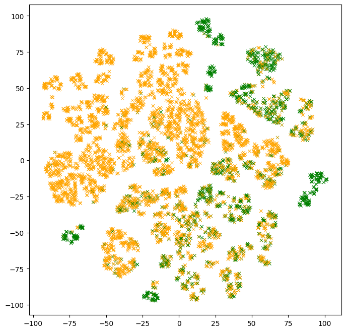
Observations:
- There are clusters of points with similar colors. Those are examples that are easy for the model to classify.
- There are multiple clusters with the same color. Those multiple clusters show examples with the same label, but for "different reasons" according to the model.
- Clusters with mixed colors contain examples where the model performs poorly. In the part above, we evaluated the model test accuracy to ~86%. Those are likely those examples.
The previous plot is a static image. Let's turn it into an interactive plot and inspect the individual examples.
# docs_infra: no_execute

# Note: Run the colab (click the "Run in Google Colab" link at the top) to see
# the interactive plot.

def interactive_plot(dataset, projections):

  def label_fn(row):
    """HTML printer over each example."""
    return "<br>".join([f"<b>{k}:</b> {v}" for k, v in row.items()])

  labels = list(dataset.apply(label_fn, axis=1).values)
  iplot({
      "data": [
          go.Scatter(
              x=projections[:, 0],
              y=projections[:, 1],
              text=labels,
              mode="markers",
              marker={
                  "color": colors,
                  "size": 3,
              })
      ],
      "layout": go.Layout(width=600, height=600, template="simple_white")
  })


interactive_plot(test_df, t_sne)
Instructions: Put the mouse pointer over some examples, and try to make sense of them. Compare them to their neighbors.
Not seeing the interactive plot?: Run the colab with this link to see the interactive plot.
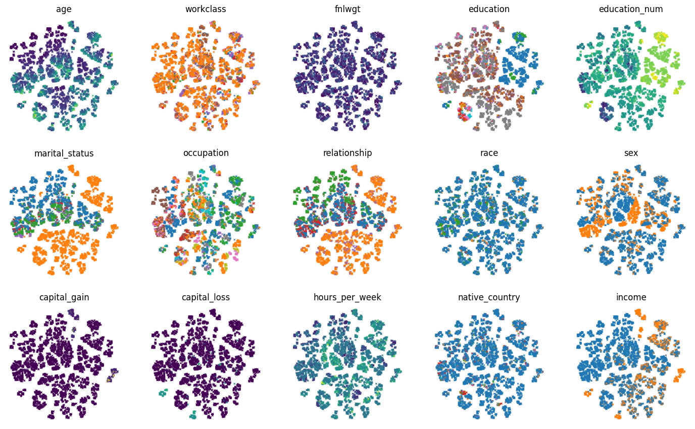
Instead of coloring the examples according to the label values, we can color the examples according to each feature values:
# Number of columns and rows in the multi-plot.
num_plot_cols = 5
num_plot_rows = math.ceil(test_df.shape[1] / num_plot_cols)

# Color palette for the categorical features.
palette = list(mcolors.TABLEAU_COLORS.values())

# Create the plot
plot_size_in = 3.5
fig, axs = plt.subplots(
    num_plot_rows,
    num_plot_cols,
    figsize=(num_plot_cols * plot_size_in, num_plot_rows * plot_size_in))

# Hide the borders.
for row in axs:
  for ax in row:
    ax.set_axis_off()

for col_idx, col_name in enumerate(test_df):
  ax = axs[col_idx // num_plot_cols, col_idx % num_plot_cols]

  colors = test_df[col_name]
  if colors.dtypes in [str, object]:
    # Use the color palette on categorical features.
    unique_values = list(colors.unique())
    colors = colors.map(
        lambda x: palette[unique_values.index(x) % len(palette)])

  ax.set_title(col_name)
  ax.scatter(t_sne[:, 0], t_sne[:, 1], c=colors.values, linewidths=0.5,
      marker="x", s=5)
Prototypes
Trying to make sense of an example by looking at all its neighbors is not always efficient. Instead, we could "group" similar examples to make this task easier. This is the underlying idea behind prototypes.
Prototypes are examples, not necessarily in the original dataset, that are representative of large trends in the dataset. Looking at prototypes is a solution to understand a dataset. For more details, see the chapter 8.7 of Interpretable Machine Learning by Molnar.
Prototypes can be computed in different ways, for example using a clustering algorithm. Instead, Breiman proposed a specific solution based on a simple iterative algorithm. The algorithm is as follow:
- Select the example surrounded with the highest number of neighbors with the same class among its k nearest neighbors.
- Create a prototype example using the median feature values of the selected example and its k neighbors.
- Remove those k+1 examples
- Repeat
Informally, prototypes are centers of clusters in the plots we created above.
Let's implement this algorithm and look at some prototypes.
First the method that selects the example in step 1.
def select_example(labels, distance_matrix, k):
  """Selects the example with the highest number of neighbors with the same class.

  Usage example:
    n = 5
    select_example(
        np.random.randint(0,2, size=n),
        np.random.uniform(size=(n,n)),
        2)

  Returns:
    The list of neighbors for the selected example. Includes the selected
    example.
  """

  partition = np.argpartition(distance_matrix, k)[:,:k]
  same_label = np.mean(np.equal(labels[partition], np.expand_dims(labels, axis=1)), axis=1)
  selected_example = np.argmax(same_label)
  return partition[selected_example, :]
def extract_prototype_examples(labels, distance_matrix, k, num_prototypes):
  """Extracts a list of examples in each prototype.

  Usage example:
    n = 50
    print(extract_prototype_examples(
        labels=np.random.randint(0, 2, size=n),
        distance_matrix=np.random.uniform(size=(n, n)),
        k=2,
        num_prototypes=3))

  Returns:
    An array where E[i][j] is the index of the j-th examples of the i-th
    prototype.
  """

  example_idxs = np.arange(len(labels))
  prototypes = []
  examples_per_prototype = []

  for iter in range(num_prototypes):
    print(f"Iter #{iter}")
    # Select the example
    neighbors = select_example(labels, distance_matrix, k)

    # Index of the examples in the prototype
    examples_per_prototype.append(list(example_idxs[neighbors]))

    # Remove the selected examples
    example_idxs = np.delete(example_idxs, neighbors)
    labels = np.delete(labels, neighbors)
    distance_matrix = np.delete(distance_matrix, neighbors, axis=0)
    distance_matrix = np.delete(distance_matrix, neighbors, axis=1)

  return examples_per_prototype
Using the methods above, let's extract the examples for 10 prototypes.
examples_per_prototype = extract_prototype_examples(test_df["income"].values, distance, k=20, num_prototypes=10)
print(f"Found examples for {len(examples_per_prototype)} prototypes.")
Iter #0
Iter #1
Iter #2
Iter #3
Iter #4
Iter #5
Iter #6
Iter #7
Iter #8
Iter #9
Found examples for 10 prototypes.
For each of those prototypes, we want to display the statistics of the feature values. In this example, we will look at the quartiles of the numerical features, and the most frequent values for the categorical features.
def build_prototype(dataset):
  """Exacts the feature statistics of a prototype.

  For numerical features, returns the quantiles.
  For categorical features, returns the most frequent value.

  Usage example:
    n = 50
    print(build_prototype(
        pd.DataFrame({
            "f1": np.random.uniform(size=n),
            "f2": np.random.uniform(size=n),
            "f3": [f"v_{x}" for x in np.random.randint(0, 2, size=n)],
            "label": np.random.randint(0, 2, size=n)
        })))

  Return:
    A prototype as a dictionary of strings.
  """

  prototype = {}
  for col in dataset.columns:
    col_values = dataset[col]
    if col_values.dtypes in [str, object]:
      # A categorical feature.

      # Remove the missing values
      col_values = [x for x in col_values if isinstance(x,str) or not math.isnan(x)]

      # Frequency of each possible value.
      frequency_item, frequency_count = np.unique(col_values, return_counts=True)
      top_item_idx = np.argmax(frequency_count)
      top_item_probability = frequency_count[top_item_idx] / np.sum(frequency_count)

      # Print the most common item.
      prototype[col] = f"{frequency_item[top_item_idx]} ({100*top_item_probability:.0f}%)"

    else:
      # A numerical feature.
      quartiles = np.nanquantile(col_values.values, [0.25, 0.5, 0.75])
      # Print the 3 quantiles.
      prototype[col] = f"{quartiles[0]} {quartiles[1]} {quartiles[2]}"
  return prototype
Now, let's look at our prototypes.
# Extract the statistics of each prototype.
prototypes = []
for examples in examples_per_prototype:
  # Prorotype statistics.
  prototypes.append(build_prototype(test_df.iloc[examples, :]))
prototypes = pd.DataFrame(prototypes)

prototypes
Try to make sense of the prototypes.
Let's extract and plot the mean 2d t-SNE projection of the elements in those prototypes.
# Extract the projection of each prototype.
prototypes_projection = []
for examples in examples_per_prototype:
  # t-SNE for each prototype.
  prototypes_projection.append(np.mean(t_sne[examples,:],axis=0))
prototypes_projection = np.stack(prototypes_projection)
# Plot the mean 2d t-SNE projection of the elements in the prototypes.

fig, ax = plt.subplots(1, 1, figsize=(8, 8))
ax.grid(False)

# Color the points according to the label value.
colors = (test_df["income"] == ">50K").map(lambda x: ["orange", "green"][x])
ax.scatter(
    t_sne[:, 0], t_sne[:, 1], c=colors, linewidths=0.5, marker="x", s=20)

# Add the prototype indices.
for i in range(prototypes_projection.shape[0]):
  ax.text(prototypes_projection[i, 0],
          prototypes_projection[i, 1],
          f"{i}",
          fontdict={"size":18},
          c="red")

We see that the 10 prototypes cover around half of the domain. Clusters of examples without a prototype would be best explained with more prototypes.
In the example above, we extracted the prototypes automatically. However, we can also build prototypes around specific examples.
Let's create the prototype around the example #0.
example_idx = 0
k = 20
neighbors = np.argpartition(distance[example_idx, :], k)[:k]

print(f"The example #{example_idx} is:")
print("===============================")
print(test_df.iloc[example_idx, :])
print("")
print(f"The prototype around the example #{example_idx} is:")
print("============================================")
print(pd.Series(build_prototype(test_df.iloc[neighbors, :])))
The example #0 is:
===============================
age                          39
workclass             State-gov
fnlwgt                    77516
education             Bachelors
education_num                13
marital_status    Never-married
occupation         Adm-clerical
relationship      Not-in-family
race                      White
sex                        Male
capital_gain               2174
capital_loss                  0
hours_per_week               40
native_country    United-States
income                    <=50K
Name: 0, dtype: object

The prototype around the example #0 is:
============================================
age                          36.0 39.0 41.0
workclass                     Private (50%)
fnlwgt            72314.0 115188.5 138797.0
education                   Bachelors (95%)
education_num                13.0 13.0 13.0
marital_status          Never-married (65%)
occupation               Adm-clerical (70%)
relationship            Not-in-family (75%)
race                            White (95%)
sex                              Male (65%)
capital_gain                    0.0 0.0 0.0
capital_loss                    0.0 0.0 0.0
hours_per_week              38.75 40.0 40.0
native_country         United-States (100%)
income                         <=50K (100%)
dtype: object