
| |
 在 GitHub 上查看源代码 在 GitHub 上查看源代码 |
梯度和自动微分简介指南包括在 TensorFlow 中计算梯度所需的全部内容。本指南重点介绍 tf.GradientTape API 更深入、更不常见的功能。
设置
import tensorflow as tf

import matplotlib as mpl
import matplotlib.pyplot as plt

mpl.rcParams['figure.figsize'] = (8, 6)
2022-12-14 22:53:27.845325: W tensorflow/compiler/xla/stream_executor/platform/default/dso_loader.cc:64] Could not load dynamic library 'libnvinfer.so.7'; dlerror: libnvinfer.so.7: cannot open shared object file: No such file or directory
2022-12-14 22:53:27.845442: W tensorflow/compiler/xla/stream_executor/platform/default/dso_loader.cc:64] Could not load dynamic library 'libnvinfer_plugin.so.7'; dlerror: libnvinfer_plugin.so.7: cannot open shared object file: No such file or directory
2022-12-14 22:53:27.845452: W tensorflow/compiler/tf2tensorrt/utils/py_utils.cc:38] TF-TRT Warning: Cannot dlopen some TensorRT libraries. If you would like to use Nvidia GPU with TensorRT, please make sure the missing libraries mentioned above are installed properly.
控制梯度记录
在自动微分指南中,您已了解构建梯度计算时如何控制条带监视变量和张量。
条带还具有操作记录的方法。
停止记录
如果您希望停止记录梯度,可以使用 tf.GradientTape.stop_recording 暂时挂起记录。
如果您不希望在模型中间对复杂运算微分,这可能有助于减少开销。其中可能包括计算指标或中间结果:
x = tf.Variable(2.0)
y = tf.Variable(3.0)

with tf.GradientTape() as t:
  x_sq = x * x
  with t.stop_recording():
    y_sq = y * y
  z = x_sq + y_sq

grad = t.gradient(z, {'x': x, 'y': y})

print('dz/dx:', grad['x'])  # 2*x => 4
print('dz/dy:', grad['y'])
dz/dx: tf.Tensor(4.0, shape=(), dtype=float32)
dz/dy: None
重置/从头开始纪录
如果您希望完全重新开始,请使用 tf.GradientTape.reset。通常,直接退出梯度带块并重新开始比较易于读取,但在退出梯度带块有困难或不可行时,可以使用 reset 方法。
x = tf.Variable(2.0)
y = tf.Variable(3.0)
reset = True

with tf.GradientTape() as t:
  y_sq = y * y
  if reset:
    # Throw out all the tape recorded so far.
    t.reset()
  z = x * x + y_sq

grad = t.gradient(z, {'x': x, 'y': y})

print('dz/dx:', grad['x'])  # 2*x => 4
print('dz/dy:', grad['y'])
dz/dx: tf.Tensor(4.0, shape=(), dtype=float32)
dz/dy: None
精确停止梯度流
与上面的全局条带控制相比,tf.stop_gradient 函数更加精确。它可以用来阻止梯度沿着特定路径流动,而不需要访问条带本身:
x = tf.Variable(2.0)
y = tf.Variable(3.0)

with tf.GradientTape() as t:
  y_sq = y**2
  z = x**2 + tf.stop_gradient(y_sq)

grad = t.gradient(z, {'x': x, 'y': y})

print('dz/dx:', grad['x'])  # 2*x => 4
print('dz/dy:', grad['y'])
dz/dx: tf.Tensor(4.0, shape=(), dtype=float32)
dz/dy: None
自定义梯度
在某些情况下,您可能需要精确控制梯度的计算方式,而不是使用默认值。这些情况包括:
- 正在编写的新运算没有定义的梯度。
- 默认计算在数值上不稳定。
- 您希望从前向传递缓存开销大的计算。
- 您想修改一个值(例如,使用
tf.clip_by_value或tf.math.round)而不修改梯度。
对于第一种情况,要编写新运算,您可以使用 tf.RegisterGradient 自行设置。(请参阅 API 文档了解详细信息)。(注意,梯度注册为全局,需谨慎更改。)
对于后三种情况,可以使用 tf.custom_gradient。
以下示例将 tf.clip_by_norm 应用于中间梯度:
# Establish an identity operation, but clip during the gradient pass.
@tf.custom_gradient
def clip_gradients(y):
  def backward(dy):
    return tf.clip_by_norm(dy, 0.5)
  return y, backward

v = tf.Variable(2.0)
with tf.GradientTape() as t:
  output = clip_gradients(v * v)
print(t.gradient(output, v))  # calls "backward", which clips 4 to 2
tf.Tensor(2.0, shape=(), dtype=float32)
请参阅 tf.custom_gradient 装饰器 API 文档,了解更多详细信息。
SavedModel 中的自定义梯度
注:此功能将从 TensorFlow 2.6 开始提供。
可以使用选项 tf.saved_model.SaveOptions(experimental_custom_gradients=True) 将自定义梯度保存到 SavedModel。
要保存到 SavedModel,梯度函数必须可以跟踪(要了解详情,请参阅使用 tf.function 提高性能指南)。
class MyModule(tf.Module):

  @tf.function(input_signature=[tf.TensorSpec(None)])
  def call_custom_grad(self, x):
    return clip_gradients(x)

model = MyModule()
tf.saved_model.save(
    model,
    'saved_model',
    options=tf.saved_model.SaveOptions(experimental_custom_gradients=True))

# The loaded gradients will be the same as the above example.
v = tf.Variable(2.0)
loaded = tf.saved_model.load('saved_model')
with tf.GradientTape() as t:
  output = loaded.call_custom_grad(v * v)
print(t.gradient(output, v))
INFO:tensorflow:Assets written to: saved_model/assets
tf.Tensor(2.0, shape=(), dtype=float32)
关于上述示例的注意事项:如果您尝试用 tf.saved_model.SaveOptions(experimental_custom_gradients=False) 替换上面的代码,梯度仍会在加载时产生相同的结果。原因在于,梯度注册表仍然包含函数 call_custom_op 中使用的自定义梯度。但是,如果在没有自定义梯度的情况下保存后重新启动运行时,则在 tf.GradientTape 下运行加载的模型会抛出错误:LookupError: No gradient defined for operation 'IdentityN' (op type: IdentityN)。
多个条带
多个条带无缝交互。
例如,下面每个条带监视不同的张量集:
x0 = tf.constant(0.0)
x1 = tf.constant(0.0)

with tf.GradientTape() as tape0, tf.GradientTape() as tape1:
  tape0.watch(x0)
  tape1.watch(x1)

  y0 = tf.math.sin(x0)
  y1 = tf.nn.sigmoid(x1)

  y = y0 + y1

  ys = tf.reduce_sum(y)
tape0.gradient(ys, x0).numpy() # cos(x) => 1.0
1.0
tape1.gradient(ys, x1).numpy() # sigmoid(x1)*(1-sigmoid(x1)) => 0.25
0.25
高阶梯度
tf.GradientTape 上下文管理器内的运算会被记录下来,以供自动微分。如果在该上下文中计算梯度,梯度计算也会被记录。因此,完全相同的 API 也适用于高阶梯度。
例如:
x = tf.Variable(1.0)  # Create a Tensorflow variable initialized to 1.0

with tf.GradientTape() as t2:
  with tf.GradientTape() as t1:
    y = x * x * x

  # Compute the gradient inside the outer `t2` context manager
  # which means the gradient computation is differentiable as well.
  dy_dx = t1.gradient(y, x)
d2y_dx2 = t2.gradient(dy_dx, x)

print('dy_dx:', dy_dx.numpy())  # 3 * x**2 => 3.0
print('d2y_dx2:', d2y_dx2.numpy())  # 6 * x => 6.0
dy_dx: 3.0
d2y_dx2: 6.0
虽然这确实可以得到标量函数的二次导数,但这种模式并不能通用于生成黑塞矩阵,因为 tf.GradientTape.gradient 只计算标量的梯度。要构造黑塞矩阵,请参见“雅可比矩阵”部分下的“黑塞矩阵”示例。
当您从梯度计算标量,然后产生的标量作为第二个梯度计算的源时,“嵌套调用 tf.GradientTape.gradient”是一种不错的模式,如以下示例所示。
示例:输入梯度正则化
许多模型都容易受到“对抗样本”影响。这种技术的集合会修改模型的输入,进而混淆模型输出。最简单的实现(例如,使用 Fast Gradient Signed Method 攻击的对抗样本)沿着输出相对于输入的梯度(即“输入梯度”) 迈出一步。
一种增强相对于对抗样本的稳健性的方法是输入梯度正则化(Finlay 和 Oberman,2019 年),这种方法会尝试将输入梯度的幅度最小化。如果输入梯度较小,那么输出的变化也应该较小。
以下是输入梯度正则化的简单实现:
- 使用内条带计算输出相对于输入的梯度。
- 计算该输入梯度的幅度。
- 计算该幅度相对于模型的梯度。
x = tf.random.normal([7, 5])

layer = tf.keras.layers.Dense(10, activation=tf.nn.relu)
with tf.GradientTape() as t2:
  # The inner tape only takes the gradient with respect to the input,
  # not the variables.
  with tf.GradientTape(watch_accessed_variables=False) as t1:
    t1.watch(x)
    y = layer(x)
    out = tf.reduce_sum(layer(x)**2)
  # 1. Calculate the input gradient.
  g1 = t1.gradient(out, x)
  # 2. Calculate the magnitude of the input gradient.
  g1_mag = tf.norm(g1)

# 3. Calculate the gradient of the magnitude with respect to the model.
dg1_mag = t2.gradient(g1_mag, layer.trainable_variables)
[var.shape for var in dg1_mag]
[TensorShape([5, 10]), TensorShape([10])]
雅可比矩阵
以上所有示例都取标量目标相对于某些源张量的梯度。
雅可比矩阵代表向量值函数的梯度。每行都包含其中一个向量元素的梯度。
tf.GradientTape.jacobian 方法让您能够有效计算雅可比矩阵。
注意:
- 类似于
gradient:sources参数可以是张量或张量的容器。 - 不同于
gradient:target张量必须是单个张量。
标量源
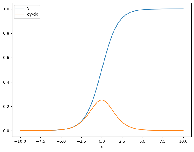
作为第一个示例,以下是矢量目标相对于标量源的雅可比矩阵。
x = tf.linspace(-10.0, 10.0, 200+1)
delta = tf.Variable(0.0)

with tf.GradientTape() as tape:
  y = tf.nn.sigmoid(x+delta)

dy_dx = tape.jacobian(y, delta)
当您相对于标量取雅可比矩阵时,结果为目标的形状,并给出每个元素相对于源的梯度:
print(y.shape)
print(dy_dx.shape)
(201,)
(201,)
plt.plot(x.numpy(), y, label='y')
plt.plot(x.numpy(), dy_dx, label='dy/dx')
plt.legend()
_ = plt.xlabel('x')
张量源
无论输入是标量还是张量,tf.GradientTape.jacobian 都能有效计算源的每个元素相对于目标的每个元素的梯度。
例如,此层的输出的形状为 (10,7)。
x = tf.random.normal([7, 5])
layer = tf.keras.layers.Dense(10, activation=tf.nn.relu)

with tf.GradientTape(persistent=True) as tape:
  y = layer(x)

y.shape
TensorShape([7, 10])
层内核的形状是 (5,10)。
layer.kernel.shape
TensorShape([5, 10])
将这两个形状连在一起就是输出相对于内核的雅可比矩阵的形状:
j = tape.jacobian(y, layer.kernel)
j.shape
TensorShape([7, 10, 5, 10])
如果您在目标的维度上求和,会得到由 tf.GradientTape.gradient 计算的总和的梯度:
g = tape.gradient(y, layer.kernel)
print('g.shape:', g.shape)

j_sum = tf.reduce_sum(j, axis=[0, 1])
delta = tf.reduce_max(abs(g - j_sum)).numpy()
assert delta < 1e-3
print('delta:', delta)
g.shape: (5, 10)
delta: 4.7683716e-07
示例:黑塞矩阵
虽然 tf.GradientTape 并没有给出构造黑塞矩阵的显式方法,但可以使用 tf.GradientTape.jacobian 方法进行构建。
注:黑塞矩阵包含 N**2 个参数。由于这个原因和其他原因,它对于大多数模型都不实际。此示例主要是为了演示如何使用 tf.GradientTape.jacobian 方法,并不是对直接黑塞矩阵优化的认可。黑塞矩阵向量积可以通过嵌套条带有效计算,这也是一种更有效的二阶优化方法。
x = tf.random.normal([7, 5])
layer1 = tf.keras.layers.Dense(8, activation=tf.nn.relu)
layer2 = tf.keras.layers.Dense(6, activation=tf.nn.relu)

with tf.GradientTape() as t2:
  with tf.GradientTape() as t1:
    x = layer1(x)
    x = layer2(x)
    loss = tf.reduce_mean(x**2)

  g = t1.gradient(loss, layer1.kernel)

h = t2.jacobian(g, layer1.kernel)
print(f'layer.kernel.shape: {layer1.kernel.shape}')
print(f'h.shape: {h.shape}')
layer.kernel.shape: (5, 8)
h.shape: (5, 8, 5, 8)
要将此黑塞矩阵用于牛顿方法步骤,首先需要将其轴展平为矩阵,然后将梯度展平为向量:
n_params = tf.reduce_prod(layer1.kernel.shape)

g_vec = tf.reshape(g, [n_params, 1])
h_mat = tf.reshape(h, [n_params, n_params])
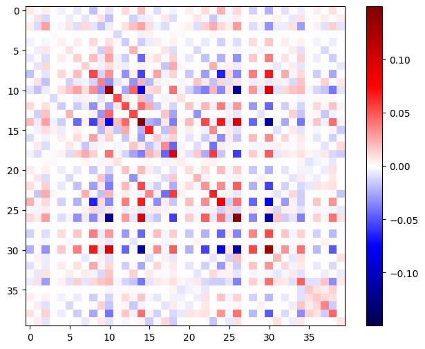
黑塞矩阵应当对称:
def imshow_zero_center(image, **kwargs):
  lim = tf.reduce_max(abs(image))
  plt.imshow(image, vmin=-lim, vmax=lim, cmap='seismic', **kwargs)
  plt.colorbar()
imshow_zero_center(h_mat)
牛顿方法更新步骤如下所示。
eps = 1e-3
eye_eps = tf.eye(h_mat.shape[0])*eps
注:实际上不反转矩阵。
# X(k+1) = X(k) - (∇²f(X(k)))^-1 @ ∇f(X(k))
# h_mat = ∇²f(X(k))
# g_vec = ∇f(X(k))
update = tf.linalg.solve(h_mat + eye_eps, g_vec)

# Reshape the update and apply it to the variable.
_ = layer1.kernel.assign_sub(tf.reshape(update, layer1.kernel.shape))
虽然这对于单个 tf.Variable 来说相对简单,但将其应用于非平凡模型则需要仔细的级联和切片,以产生跨多个变量的完整黑塞矩阵。
批量雅可比矩阵
在某些情况下,您需要取各个目标堆栈相对于源堆栈的雅可比矩阵,其中每个目标-源对的雅可比矩阵都是独立的。
例如,此处的输入 x 形状为 (batch, ins) ,输出 y 形状为 (batch, outs):
x = tf.random.normal([7, 5])

layer1 = tf.keras.layers.Dense(8, activation=tf.nn.elu)
layer2 = tf.keras.layers.Dense(6, activation=tf.nn.elu)

with tf.GradientTape(persistent=True, watch_accessed_variables=False) as tape:
  tape.watch(x)
  y = layer1(x)
  y = layer2(y)

y.shape
TensorShape([7, 6])
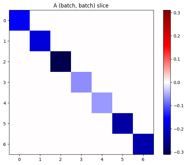
y 相对 x 的完整雅可比矩阵的形状为 (batch, ins, batch, outs),即使您只想要 (batch, ins, outs)。
j = tape.jacobian(y, x)
j.shape
TensorShape([7, 6, 7, 5])
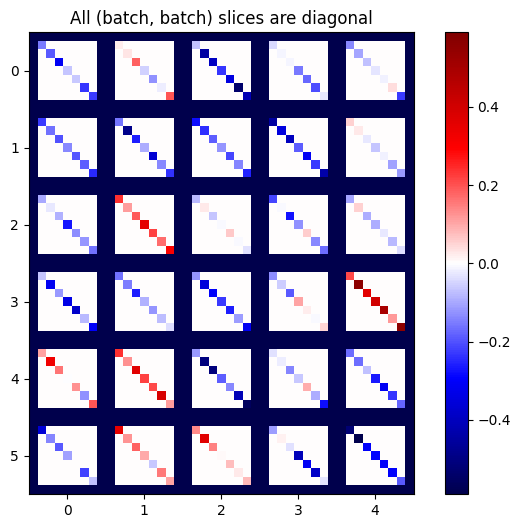
如果堆栈中各项的梯度相互独立,那么此张量的每一个 (batch, batch) 切片都是对角矩阵:
imshow_zero_center(j[:, 0, :, 0])
_ = plt.title('A (batch, batch) slice')
def plot_as_patches(j):
  # Reorder axes so the diagonals will each form a contiguous patch.
  j = tf.transpose(j, [1, 0, 3, 2])
  # Pad in between each patch.
  lim = tf.reduce_max(abs(j))
  j = tf.pad(j, [[0, 0], [1, 1], [0, 0], [1, 1]],
             constant_values=-lim)
  # Reshape to form a single image.
  s = j.shape
  j = tf.reshape(j, [s[0]*s[1], s[2]*s[3]])
  imshow_zero_center(j, extent=[-0.5, s[2]-0.5, s[0]-0.5, -0.5])

plot_as_patches(j)
_ = plt.title('All (batch, batch) slices are diagonal')
要获取所需结果,您可以对重复的 batch 维度求和,或者使用 tf.einsum 选择对角线:
j_sum = tf.reduce_sum(j, axis=2)
print(j_sum.shape)
j_select = tf.einsum('bxby->bxy', j)
print(j_select.shape)
(7, 6, 5)
(7, 6, 5)
没有额外维度时,计算会更加高效。tf.GradientTape.batch_jacobian 方法就是如此运作的:
jb = tape.batch_jacobian(y, x)
jb.shape
WARNING:tensorflow:5 out of the last 5 calls to <function pfor.<locals>.f at 0x7f85281da0d0> triggered tf.function retracing. Tracing is expensive and the excessive number of tracings could be due to (1) creating @tf.function repeatedly in a loop, (2) passing tensors with different shapes, (3) passing Python objects instead of tensors. For (1), please define your @tf.function outside of the loop. For (2), @tf.function has reduce_retracing=True option that can avoid unnecessary retracing. For (3), please refer to https://www.tensorflow.org/guide/function#controlling_retracing and https://www.tensorflow.org/api_docs/python/tf/function for  more details.
TensorShape([7, 6, 5])
error = tf.reduce_max(abs(jb - j_sum))
assert error < 1e-3
print(error.numpy())
0.0
小心:tf.GradientTape.batch_jacobian 只验证源和目标的第一维是否匹配,并不会检查梯度是否独立。用户需要确保仅在合理条件下使用 batch_jacobian。例如,添加 tf.keras.layers.BatchNormalization 将破坏独立性,因为它在 batch 维度进行了归一化:
x = tf.random.normal([7, 5])

layer1 = tf.keras.layers.Dense(8, activation=tf.nn.elu)
bn = tf.keras.layers.BatchNormalization()
layer2 = tf.keras.layers.Dense(6, activation=tf.nn.elu)

with tf.GradientTape(persistent=True, watch_accessed_variables=False) as tape:
  tape.watch(x)
  y = layer1(x)
  y = bn(y, training=True)
  y = layer2(y)

j = tape.jacobian(y, x)
print(f'j.shape: {j.shape}')
WARNING:tensorflow:6 out of the last 6 calls to <function pfor.<locals>.f at 0x7f85a003df70> triggered tf.function retracing. Tracing is expensive and the excessive number of tracings could be due to (1) creating @tf.function repeatedly in a loop, (2) passing tensors with different shapes, (3) passing Python objects instead of tensors. For (1), please define your @tf.function outside of the loop. For (2), @tf.function has reduce_retracing=True option that can avoid unnecessary retracing. For (3), please refer to https://www.tensorflow.org/guide/function#controlling_retracing and https://www.tensorflow.org/api_docs/python/tf/function for  more details.
j.shape: (7, 6, 7, 5)
plot_as_patches(j)

_ = plt.title('These slices are not diagonal')
_ = plt.xlabel("Don't use `batch_jacobian`")
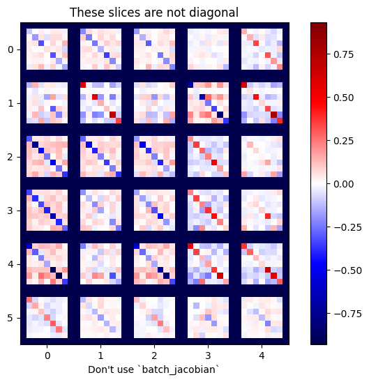
在此示例中,batch_jacobian 仍然可以运行并返回某些信息与预期形状,但其内容具有不明确的含义:
jb = tape.batch_jacobian(y, x)
print(f'jb.shape: {jb.shape}')
jb.shape: (7, 6, 5)