
| |
 GitHub에서 소스 보기 GitHub에서 소스 보기 |
이전 가이드에서 텐서, 변수, 그래디언트 테이프 , 모듈에 관해 배웠습니다. 이 가이드에서는 모델을 훈련하기 위해 이들 요소를 모두 맞춤 조정합니다.
TensorFlow에는 상용구를 줄이기 위해 유용한 추상화를 제공하는 상위 수준의 신경망 API인 tf.Keras API도 포함되어 있습니다. 그러나 이 가이드에서는 기본 클래스를 사용합니다.
설정
import tensorflow as tf

import matplotlib.pyplot as plt

colors = plt.rcParams['axes.prop_cycle'].by_key()['color']
2022-12-14 21:14:34.737656: W tensorflow/compiler/xla/stream_executor/platform/default/dso_loader.cc:64] Could not load dynamic library 'libnvinfer.so.7'; dlerror: libnvinfer.so.7: cannot open shared object file: No such file or directory
2022-12-14 21:14:34.737744: W tensorflow/compiler/xla/stream_executor/platform/default/dso_loader.cc:64] Could not load dynamic library 'libnvinfer_plugin.so.7'; dlerror: libnvinfer_plugin.so.7: cannot open shared object file: No such file or directory
2022-12-14 21:14:34.737753: W tensorflow/compiler/tf2tensorrt/utils/py_utils.cc:38] TF-TRT Warning: Cannot dlopen some TensorRT libraries. If you would like to use Nvidia GPU with TensorRT, please make sure the missing libraries mentioned above are installed properly.
머신러닝 문제 해결하기
머신러닝 문제의 해결은 일반적으로 다음 단계로 구성됩니다.
- 훈련 데이터를 얻습니다.
- 모델을 정의합니다.
- 손실 함수를 정의합니다.
- 훈련 데이터를 실행하여 이상적인 값에서 손실을 계산합니다.
- 손실에 대한 기울기를 계산하고 최적화 프로그램 를 사용하여 데이터에 맞게 변수를 조정합니다.
- 결과를 평가합니다.
설명을 위해 이 가이드에서는 \(W\)(가중치) 및 \(b\)(바이어스)의 두 가지 변수가 있는 간단한 선형 모델 \(f(x) = x * W + b\)를 개발합니다.
이것이 가장 기본적인 머신러닝 문제입니다. \(x\)와 \(y\)가 주어지면 간단한 선형 회귀를 통해 선의 기울기와 오프셋을 찾습니다.
데이터
지도 학습은 입력(일반적으로 x로 표시됨)과 출력(y로 표시, 종종 레이블이라고 함)을 사용합니다. 목표는 입력에서 출력 값을 예측할 수 있도록 쌍을 이룬 입력과 출력에서 학습하는 것입니다.
TensorFlow에서 데이터의 각 입력은 거의 항상 텐서로 표현되며, 종종 벡터입니다. 지도 학습에서 출력(또는 예측하려는 값)도 텐서입니다.
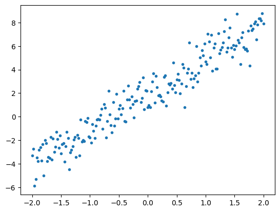
다음은 선을 따라 점에 가우시안 (정규 분포) 노이즈를 추가하여 합성된 데이터입니다.
# The actual line
TRUE_W = 3.0
TRUE_B = 2.0

NUM_EXAMPLES = 201

# A vector of random x values
x = tf.linspace(-2,2, NUM_EXAMPLES)
x = tf.cast(x, tf.float32)

def f(x):
  return x * TRUE_W + TRUE_B

# Generate some noise
noise = tf.random.normal(shape=[NUM_EXAMPLES])

# Calculate y
y = f(x) + noise
# Plot all the data
plt.plot(x, y, '.')
plt.show()
텐서는 일반적으로 배치 또는 입력과 출력이 함께 쌓인 그룹의 형태로 수집됩니다. 일괄 처리는 몇 가지 훈련 이점을 제공할 수 있으며 가속기 및 벡터화된 계산에서 잘 동작합니다. 데이터세트가 얼마나 작은지를 고려할 때 전체 데이터세트를 단일 배치로 처리할 수 있습니다.
모델 정의하기
tf.Variable을 사용하여 모델의 모든 가중치를 나타냅니다. tf.Variable은 값을 저장하고 필요에 따라 텐서 형식으로 제공합니다. 자세한 내용은 변수 가이드를 참조하세요.
tf.Module을 사용하여 변수와 계산을 캡슐화합니다. 모든 Python 객체를 사용할 수 있지만 이렇게 하면 쉽게 저장할 수 있습니다.
여기서 w와 b를 모두 변수로 정의합니다.
class MyModel(tf.Module):
  def __init__(self, **kwargs):
    super().__init__(**kwargs)
    # Initialize the weights to `5.0` and the bias to `0.0`
    # In practice, these should be randomly initialized
    self.w = tf.Variable(5.0)
    self.b = tf.Variable(0.0)

  def __call__(self, x):
    return self.w * x + self.b

model = MyModel()

# List the variables tf.modules's built-in variable aggregation.
print("Variables:", model.variables)

# Verify the model works
assert model(3.0).numpy() == 15.0
Variables: (<tf.Variable 'Variable:0' shape=() dtype=float32, numpy=0.0>, <tf.Variable 'Variable:0' shape=() dtype=float32, numpy=5.0>)
초기 변수는 여기에서 고정된 방식으로 설정되지만 Keras에는 나머지 Keras의 유무에 관계없이 사용할 수 있는 여러 초기화 프로그램이 함께 제공됩니다.
손실 함수 정의하기
손실 함수는 주어진 입력에 대한 모델의 출력이 목표 출력과 얼마나 잘 일치하는지 측정합니다. 목표는 훈련 중에 이러한 차이를 최소화하는 것입니다. "평균 제곱" 오류라고도 하는 표준 L2 손실을 정의합니다.
# This computes a single loss value for an entire batch
def loss(target_y, predicted_y):
  return tf.reduce_mean(tf.square(target_y - predicted_y))
모델을 훈련하기 전에 모델의 예측을 빨간색으로, 훈련 데이터를 파란색으로 플롯하여 손실값을 시각화할 수 있습니다.
plt.plot(x, y, '.', label="Data")
plt.plot(x, f(x), label="Ground truth")
plt.plot(x, model(x), label="Predictions")
plt.legend()
plt.show()

print("Current loss: %1.6f" % loss(y, model(x)).numpy())
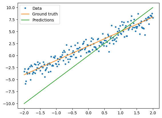
Current loss: 10.288067
훈련 루프 정의하기
훈련 루프는 순서대로 3가지 작업을 반복적으로 수행하는 것으로 구성됩니다.
- 모델을 통해 입력 배치를 전송하여 출력 생성
- 출력을 출력(또는 레이블)과 비교하여 손실 계산
- 그래디언트 테이프를 사용하여 그래디언트 찾기
- 해당 그래디언트로 변수 최적화
이 예제에서는 경사 하강법을 사용하여 모델을 훈련할 수 있습니다.
tf.keras.optimizers에서 캡처되는 경사 하강법 체계에는 다양한 변형이 있습니다. 하지만 첫 번째 원칙을 준수하는 의미에서, 기본적인 수학을 직접 구현할 것입니다. 자동 미분을 위한 tf.GradientTape 및 값 감소를 위한 tf.assign_sub(tf.assign과 tf.sub를 결합하는 값)의 도움을 받습니다.
# Given a callable model, inputs, outputs, and a learning rate...
def train(model, x, y, learning_rate):

  with tf.GradientTape() as t:
    # Trainable variables are automatically tracked by GradientTape
    current_loss = loss(y, model(x))

  # Use GradientTape to calculate the gradients with respect to W and b
  dw, db = t.gradient(current_loss, [model.w, model.b])

  # Subtract the gradient scaled by the learning rate
  model.w.assign_sub(learning_rate * dw)
  model.b.assign_sub(learning_rate * db)
훈련을 살펴보려면 훈련 루프를 통해 x 및 y의 같은 배치를 보내고 W 및 b가 발전하는 모양을 확인합니다.
model = MyModel()

# Collect the history of W-values and b-values to plot later
weights = []
biases = []
epochs = range(10)

# Define a training loop
def report(model, loss):
  return f"W = {model.w.numpy():1.2f}, b = {model.b.numpy():1.2f}, loss={loss:2.5f}"


def training_loop(model, x, y):

  for epoch in epochs:
    # Update the model with the single giant batch
    train(model, x, y, learning_rate=0.1)

    # Track this before I update
    weights.append(model.w.numpy())
    biases.append(model.b.numpy())
    current_loss = loss(y, model(x))

    print(f"Epoch {epoch:2d}:")
    print("    ", report(model, current_loss))
훈련 수행
current_loss = loss(y, model(x))

print(f"Starting:")
print("    ", report(model, current_loss))

training_loop(model, x, y)
Starting:
     W = 5.00, b = 0.00, loss=10.28807
Epoch  0:
     W = 4.45, b = 0.38, loss=6.35338
Epoch  1:
     W = 4.04, b = 0.68, loss=4.11694
Epoch  2:
     W = 3.75, b = 0.92, loss=2.83603
Epoch  3:
     W = 3.53, b = 1.11, loss=2.09655
Epoch  4:
     W = 3.37, b = 1.27, loss=1.66616
Epoch  5:
     W = 3.26, b = 1.39, loss=1.41360
Epoch  6:
     W = 3.17, b = 1.49, loss=1.26418
Epoch  7:
     W = 3.11, b = 1.57, loss=1.17507
Epoch  8:
     W = 3.07, b = 1.63, loss=1.12153
Epoch  9:
     W = 3.03, b = 1.68, loss=1.08912
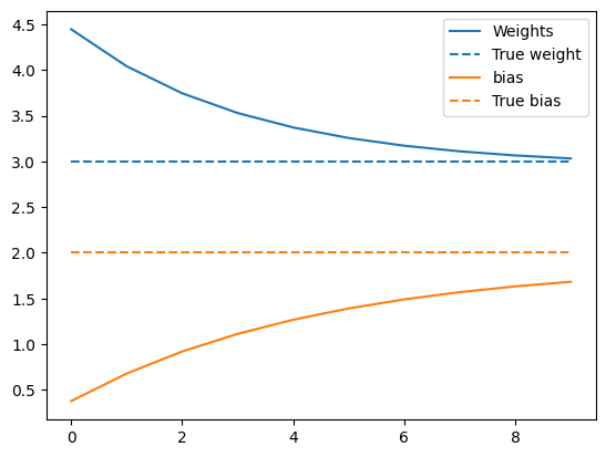
시간이 지남에 따른 가중치의 전개 양상을 표시:
plt.plot(epochs, weights, label='Weights', color=colors[0])
plt.plot(epochs, [TRUE_W] * len(epochs), '--',
         label = "True weight", color=colors[0])

plt.plot(epochs, biases, label='bias', color=colors[1])
plt.plot(epochs, [TRUE_B] * len(epochs), "--",
         label="True bias", color=colors[1])

plt.legend()
plt.show()
훈련된 모델 성능 시각화
plt.plot(x, y, '.', label="Data")
plt.plot(x, f(x), label="Ground truth")
plt.plot(x, model(x), label="Predictions")
plt.legend()
plt.show()

print("Current loss: %1.6f" % loss(model(x), y).numpy())
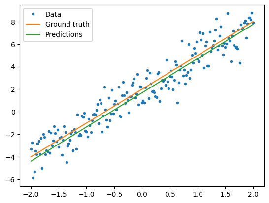
Current loss: 1.089116
같은 솔루션이지만, Keras를 사용한 경우
위의 코드를 Keras의 해당 코드와 대조해 보면 유용합니다.
tf.keras.Model을 하위 클래스화하면 모델 정의는 정확히 같게 보입니다. Keras 모델은 궁극적으로 모듈에서 상속한다는 것을 기억하세요.
class MyModelKeras(tf.keras.Model):
  def __init__(self, **kwargs):
    super().__init__(**kwargs)
    # Initialize the weights to `5.0` and the bias to `0.0`
    # In practice, these should be randomly initialized
    self.w = tf.Variable(5.0)
    self.b = tf.Variable(0.0)

  def call(self, x):
    return self.w * x + self.b

keras_model = MyModelKeras()

# Reuse the training loop with a Keras model
training_loop(keras_model, x, y)

# You can also save a checkpoint using Keras's built-in support
keras_model.save_weights("my_checkpoint")
Epoch  0:
     W = 4.45, b = 0.38, loss=6.35338
Epoch  1:
     W = 4.04, b = 0.68, loss=4.11694
Epoch  2:
     W = 3.75, b = 0.92, loss=2.83603
Epoch  3:
     W = 3.53, b = 1.11, loss=2.09655
Epoch  4:
     W = 3.37, b = 1.27, loss=1.66616
Epoch  5:
     W = 3.26, b = 1.39, loss=1.41360
Epoch  6:
     W = 3.17, b = 1.49, loss=1.26418
Epoch  7:
     W = 3.11, b = 1.57, loss=1.17507
Epoch  8:
     W = 3.07, b = 1.63, loss=1.12153
Epoch  9:
     W = 3.03, b = 1.68, loss=1.08912
모델을 생성할 때마다 새로운 훈련 루프를 작성하는 대신 Keras의 내장 기능을 바로 가기로 사용할 수 있습니다. Python 훈련 루프를 작성하거나 디버그하지 않으려는 경우 유용할 수 있습니다.
그렇게 하려면, model.compile()을 사용하여 매개변수를 설정하고 model.fit()을 사용하여 훈련해야 합니다. L2 손실 및 경사 하강법의 Keras 구현을 바로 가기로 사용하면 코드가 적을 수 있습니다. Keras 손실 및 최적화 프록그램은 이러한 편의성 함수 외부에서 사용할 수 있으며 이전 예제에서 사용할 수 있습니다.
keras_model = MyModelKeras()

# compile sets the training parameters
keras_model.compile(
    # By default, fit() uses tf.function().  You can
    # turn that off for debugging, but it is on now.
    run_eagerly=False,

    # Using a built-in optimizer, configuring as an object
    optimizer=tf.keras.optimizers.SGD(learning_rate=0.1),

    # Keras comes with built-in MSE error
    # However, you could use the loss function
    # defined above
    loss=tf.keras.losses.mean_squared_error,
)
Keras fit 배치 데이터 또는 전체 데이터세트를 NumPy 배열로 예상합니다. NumPy 배열은 배치로 분할되며, 기본 배치 크기는 32입니다.
이 경우 손으로 쓴 루프의 동작과 일치시키려면 x를 크기 1000의 단일 배치로 전달해야 합니다.
print(x.shape[0])
keras_model.fit(x, y, epochs=10, batch_size=1000)
201
Epoch 1/10
1/1 [==============================] - 0s 366ms/step - loss: 10.2881
Epoch 2/10
1/1 [==============================] - 0s 5ms/step - loss: 6.3534
Epoch 3/10
1/1 [==============================] - 0s 4ms/step - loss: 4.1169
Epoch 4/10
1/1 [==============================] - 0s 4ms/step - loss: 2.8360
Epoch 5/10
1/1 [==============================] - 0s 4ms/step - loss: 2.0966
Epoch 6/10
1/1 [==============================] - 0s 4ms/step - loss: 1.6662
Epoch 7/10
1/1 [==============================] - 0s 4ms/step - loss: 1.4136
Epoch 8/10
1/1 [==============================] - 0s 4ms/step - loss: 1.2642
Epoch 9/10
1/1 [==============================] - 0s 4ms/step - loss: 1.1751
Epoch 10/10
1/1 [==============================] - 0s 4ms/step - loss: 1.1215
<keras.callbacks.History at 0x7f91c022fe80>
Keras는 훈련 전이 아닌 훈련 후 손실을 출력하므로 첫 번째 손실이 더 낮게 나타나지만, 그렇지 않으면 본질적으로 같은 훈련 성능을 보여줍니다.
다음 단계
이 가이드에서는 텐서, 변수, 모듈 및 그래디언트 테이프의 핵심 클래스를 사용하여 모델을 빌드하고 훈련하는 방법과 이러한 아이디어가 Keras에 매핑되는 방법을 살펴보았습니다.
그러나 이것은 매우 단순한 문제입니다. 보다 실용적인 소개는 사용자 정의 훈련 연습을 참조하세요.
내장 Keras 훈련 루프의 사용에 관한 자세한 내용은 이 가이드를 참조하세요. 훈련 루프 및 Keras에 관한 자세한 내용은 이 가이드를 참조하세요. 사용자 정의 분산 훈련 루프의 작성에 관해서는 이 가이드를 참조하세요.