
| |
 GitHub에서 소스 보기 GitHub에서 소스 보기 |
tf.data API를 사용하면 간단하고 재사용 가능한 조각으로 복잡한 입력 파이프라인을 빌드할 수 있습니다. 예를 들어, 이미지 모델의 파이프라인은 분산된 파일 시스템의 파일에서 데이터를 집계하고 각 이미지에 임의의 퍼터베이션을 적용하며 무작위로 선택한 이미지를 학습을 위한 batch로 병합할 수 있습니다. 텍스트 모델의 파이프라인에는 원시 텍스트 데이터에서 심볼을 추출하고, 이를 룩업 테이블이 있는 embedding 식별자로 변환하며, 길이가 서로 다른 시퀀스를 batch 처리하는 과정이 포함될 수 있습니다. tf.data API를 사용하면 많은 양의 데이터를 처리하고 여러 데이터 형식에서 데이터를 읽으며 복잡한 변환을 수행할 수 있습니다.
tf.data API는 일련의 요소를 나타내는 tf.data.Dataset 추상화를 도입하며, 여기서 각 요소는 하나 이상의 구성 요소로 이루어집니다. 예를 들어, 이미지 파이프라인에서 요소는 이미지와 해당 label을 나타내는 텐서 구성 요소 쌍이 있는 단일 학습 예일 수 있습니다.
데이터 세트를 생성하는 방법에는 두 가지가 있습니다.
데이터 소스는 메모리 또는 하나 이상의 파일에 저장된 데이터로부터
Dataset를 구성합니다.데이터 변환은 하나 이상의
tf.data.Dataset객체로부터 데이터세트를 구성합니다.
import tensorflow as tf
2022-12-14 22:04:10.000151: W tensorflow/compiler/xla/stream_executor/platform/default/dso_loader.cc:64] Could not load dynamic library 'libnvinfer.so.7'; dlerror: libnvinfer.so.7: cannot open shared object file: No such file or directory
2022-12-14 22:04:10.000238: W tensorflow/compiler/xla/stream_executor/platform/default/dso_loader.cc:64] Could not load dynamic library 'libnvinfer_plugin.so.7'; dlerror: libnvinfer_plugin.so.7: cannot open shared object file: No such file or directory
2022-12-14 22:04:10.000248: W tensorflow/compiler/tf2tensorrt/utils/py_utils.cc:38] TF-TRT Warning: Cannot dlopen some TensorRT libraries. If you would like to use Nvidia GPU with TensorRT, please make sure the missing libraries mentioned above are installed properly.
import pathlib
import os
import matplotlib.pyplot as plt
import pandas as pd
import numpy as np

np.set_printoptions(precision=4)
기본 메커니즘
입력 파이프라인을 만들려면 데이터 소스로 시작해야 합니다. 예를 들어 메모리의 데이터에서 Dataset를 구성하려면 tf.data.Dataset.from_tensors() 또는 tf.data.Dataset.from_tensor_slices()을 사용할 수 있습니다. 또는 입력 데이터가 권장 TFRecord 형식으로 파일에 저장된 경우 tf.data.TFRecordDataset()를 사용할 수 있습니다.
Dataset 객체가 있으면 tf.data.Dataset 객체의 메서드 호출을 연결하여 새로운 Dataset로 변환할 수 있습니다. 예를 들어 Dataset.map과 같은 요소 별 변환과 Dataset.batch와 같은 다중 요소 변환을 적용할 수 있습니다. 전체 변환 목록은 tf.data.Dataset 설명서를 참고하십시오.
Dataset 객체는 Python 반복 가능합니다. 이를 통해 for 루프를 이용해 해당 요소를 소비할 수 있습니다.
dataset = tf.data.Dataset.from_tensor_slices([8, 3, 0, 8, 2, 1])
dataset
<TensorSliceDataset element_spec=TensorSpec(shape=(), dtype=tf.int32, name=None)>
for elem in dataset:
  print(elem.numpy())
8
3
0
8
2
1
또는 iter를 사용하여 명시적으로 Python 반복기(iterator)를 작성하고 next를 사용하여 해당 요소를 소비할 수 있습니다.
it = iter(dataset)

print(next(it).numpy())
8
아니면 reduce 변환을 사용하여 데이터세트 요소를 소비할 수도 있습니다. 이렇게 하면 모든 요소가 줄어들어 단일 결과가 생성됩니다. 다음 예제는 reduce 변환을 사용하여 정수 데이터세트의 합계를 계산하는 방법을 보여줍니다.
print(dataset.reduce(0, lambda state, value: state + value).numpy())
WARNING:tensorflow:From /tmpfs/src/tf_docs_env/lib/python3.9/site-packages/tensorflow/python/autograph/pyct/static_analysis/liveness.py:83: Analyzer.lamba_check (from tensorflow.python.autograph.pyct.static_analysis.liveness) is deprecated and will be removed after 2023-09-23.
Instructions for updating:
Lambda fuctions will be no more assumed to be used in the statement where they are used, or at least in the same block. https://github.com/tensorflow/tensorflow/issues/56089
22
데이터세트 구조
데이터세트는 각 요소가 동일한 구성 요소 (중첩) 구조를 갖는 요소의 시퀀스를 생성합니다. 구조의 개별 구성 요소는 tf.TypeSpec에 의해 표현되는 어떤 유형일 수도 있으며, 여기에는 tf.Tensor, tf.sparse.SparseTensor, tf.RaggedTensor, tf.TensorArray 또는 tf.data.Dataset가 포함됩니다.
요소의 (중첩된) 구조를 표현하는 데 사용할 수 있는 Python 구조에는 tuple, dict, NamedTuple 및 OrderedDict가 있습니다. 특히 list는 데이터세트 요소의 구조를 표현하는 데 유효한 구조가 아닙니다. 이는 초기 tf.data 사용자들이 list 입력이 자동으로 텐서로 압축(예: tf.data.Dataset.from_tensors로 전달될 경우)되고 list 출력이 tuple로 강제 변환(예: 사용자 정의 함수의 반환 값)되는 부분을 강하게 느꼈기 때문입니다. 결과적으로 list 입력을 구조로 처리하려면 이를 tuple로 변환해야 하며 list 출력이 단일 구성 요소가 되도록 하려면 tf.stack을 사용하여 이를 명시적으로 구성해야 합니다.
Dataset.element_spec 속성을 사용하면 각 요소의 구성 요소 유형을 검사할 수 있습니다. 이 속성은 단일 구성 요소, 구성 요소의 튜플 또는 구성 요소의 중첩된 튜플일 수 있는 요소의 구조와 일치하는 tf.TypeSpec 객체의 중첩 구조를 반환합니다. 예를 들면 다음과 같습니다.
dataset1 = tf.data.Dataset.from_tensor_slices(tf.random.uniform([4, 10]))

dataset1.element_spec
TensorSpec(shape=(10,), dtype=tf.float32, name=None)
dataset2 = tf.data.Dataset.from_tensor_slices(
   (tf.random.uniform([4]),
    tf.random.uniform([4, 100], maxval=100, dtype=tf.int32)))

dataset2.element_spec
(TensorSpec(shape=(), dtype=tf.float32, name=None),
 TensorSpec(shape=(100,), dtype=tf.int32, name=None))
dataset3 = tf.data.Dataset.zip((dataset1, dataset2))

dataset3.element_spec
(TensorSpec(shape=(10,), dtype=tf.float32, name=None),
 (TensorSpec(shape=(), dtype=tf.float32, name=None),
  TensorSpec(shape=(100,), dtype=tf.int32, name=None)))
# Dataset containing a sparse tensor.
dataset4 = tf.data.Dataset.from_tensors(tf.SparseTensor(indices=[[0, 0], [1, 2]], values=[1, 2], dense_shape=[3, 4]))

dataset4.element_spec
SparseTensorSpec(TensorShape([3, 4]), tf.int32)
# Use value_type to see the type of value represented by the element spec
dataset4.element_spec.value_type
tensorflow.python.framework.sparse_tensor.SparseTensor
Dataset 변환은 모든 구조의 데이터세트를 지원합니다. 각 요소에 함수를 적용하는 Dataset.map 및 Dataset.filter 변환을 사용하는 경우 요소 구조에 따라 함수의 인수가 결정됩니다.
dataset1 = tf.data.Dataset.from_tensor_slices(
    tf.random.uniform([4, 10], minval=1, maxval=10, dtype=tf.int32))

dataset1
<TensorSliceDataset element_spec=TensorSpec(shape=(10,), dtype=tf.int32, name=None)>
for z in dataset1:
  print(z.numpy())
[6 5 2 4 7 4 7 7 4 5]
[1 4 5 5 5 8 2 8 1 8]
[3 3 3 4 8 4 3 8 3 9]
[5 9 1 2 7 6 5 3 6 8]
dataset2 = tf.data.Dataset.from_tensor_slices(
   (tf.random.uniform([4]),
    tf.random.uniform([4, 100], maxval=100, dtype=tf.int32)))

dataset2
<TensorSliceDataset element_spec=(TensorSpec(shape=(), dtype=tf.float32, name=None), TensorSpec(shape=(100,), dtype=tf.int32, name=None))>
dataset3 = tf.data.Dataset.zip((dataset1, dataset2))

dataset3
<ZipDataset element_spec=(TensorSpec(shape=(10,), dtype=tf.int32, name=None), (TensorSpec(shape=(), dtype=tf.float32, name=None), TensorSpec(shape=(100,), dtype=tf.int32, name=None)))>
for a, (b,c) in dataset3:
  print('shapes: {a.shape}, {b.shape}, {c.shape}'.format(a=a, b=b, c=c))
shapes: (10,), (), (100,)
shapes: (10,), (), (100,)
shapes: (10,), (), (100,)
shapes: (10,), (), (100,)
입력 데이터 읽기
NumPy 배열 소비
자세한 예는 NumPy 배열 로드 튜토리얼을 참고하세요.
모든 입력 데이터가 메모리에 맞는 경우, 여기서 Dataset를 생성하는 가장 간단한 방법은 이를 tf.Tensor 객체로 변환하고 Dataset.from_tensor_slices를 사용하는 것입니다.
train, test = tf.keras.datasets.fashion_mnist.load_data()
Downloading data from https://storage.googleapis.com/tensorflow/tf-keras-datasets/train-labels-idx1-ubyte.gz
29515/29515 [==============================] - 0s 0us/step
Downloading data from https://storage.googleapis.com/tensorflow/tf-keras-datasets/train-images-idx3-ubyte.gz
26421880/26421880 [==============================] - 0s 0us/step
Downloading data from https://storage.googleapis.com/tensorflow/tf-keras-datasets/t10k-labels-idx1-ubyte.gz
5148/5148 [==============================] - 0s 0us/step
Downloading data from https://storage.googleapis.com/tensorflow/tf-keras-datasets/t10k-images-idx3-ubyte.gz
4422102/4422102 [==============================] - 0s 0us/step
images, labels = train
images = images/255

dataset = tf.data.Dataset.from_tensor_slices((images, labels))
dataset
<TensorSliceDataset element_spec=(TensorSpec(shape=(28, 28), dtype=tf.float64, name=None), TensorSpec(shape=(), dtype=tf.uint8, name=None))>
참고: 위의 코드 조각은 features 및 labels 배열을 tf.constant() 연산으로 TensorFlow 그래프에 임베딩 처리합니다. 작은 데이터세트일 때는 효과적이지만, 배열의 내용이 여러 번 복사되기 때문에 메모리가 낭비되어 tf.GraphDef 프로토콜 버퍼의 2GB 제한에 도달할 수 있습니다.
Python generator 소비
tf.data.Dataset로 쉽게 수집할 수 있는 또 다른 일반적인 데이터 소스는 Python 생성기(generator)입니다.
주의: 이 방법은 편리한 방법이지만 이식성과 확장성이 제한적입니다. 생성기를 생성한 것과 동일한 Python 프로세스에서 실행해야 하며 계속 Python GIL의 영향을 받습니다.
def count(stop):
  i = 0
  while i<stop:
    yield i
    i += 1
for n in count(5):
  print(n)
0
1
2
3
4
Dataset.from_generator 생성자(constructor)는 Python 생성기를 완벽하게 작동하는 tf.data.Dataset로 변환합니다.
이 생성자는 반복기가 아니라 callable을 입력으로 사용합니다. 이를 통해 생성기가 끝에 도달하면 다시 시작할 수 있습니다. callable의 인수로 전달되는 args 인수가 선택적으로 사용됩니다.
tf.data가 tf.Graph를 내부적으로 빌드하고 그래프 엣지에 tf.dtype가 필요하기 때문에 output_types 인수가 필요합니다.
ds_counter = tf.data.Dataset.from_generator(count, args=[25], output_types=tf.int32, output_shapes = (), )
for count_batch in ds_counter.repeat().batch(10).take(10):
  print(count_batch.numpy())
[0 1 2 3 4 5 6 7 8 9]
[10 11 12 13 14 15 16 17 18 19]
[20 21 22 23 24  0  1  2  3  4]
[ 5  6  7  8  9 10 11 12 13 14]
[15 16 17 18 19 20 21 22 23 24]
[0 1 2 3 4 5 6 7 8 9]
[10 11 12 13 14 15 16 17 18 19]
[20 21 22 23 24  0  1  2  3  4]
[ 5  6  7  8  9 10 11 12 13 14]
[15 16 17 18 19 20 21 22 23 24]
output_shapes 인수는 필요 하지 않지만 많은 TensorFlow 연산이 알 수없는 순위의 텐서를 지원하지 않으므로 사용이 권장됩니다. 특정 축의 길이를 알 수 없거나 가변적인 경우 output_shapes에서 None으로 설정하십시오.
output_shapes 및 output_types가 다른 데이터세트 메서드와 동일한 중첩 규칙을 따른다는 점도 알고 있어야 합니다.
다음은 두 가지 측면을 모두 보여주는 예제 생성기입니다. 두 배열은 길이가 알려지지 않은 벡터입니다.
def gen_series():
  i = 0
  while True:
    size = np.random.randint(0, 10)
    yield i, np.random.normal(size=(size,))
    i += 1
for i, series in gen_series():
  print(i, ":", str(series))
  if i > 5:
    break
0 : [-0.0993 -0.1054]
1 : [ 1.0119  0.5846 -0.4908]
2 : [-0.2593  0.1929  1.4978 -1.279 ]
3 : [-0.2179 -1.0681 -1.1471 -1.6119]
4 : [ 1.0698  0.7929 -0.462   0.3334  0.3197 -0.1836]
5 : [-0.6459  0.4946  1.1721 -1.1227  0.9971 -0.2345 -1.2515 -0.448  -1.2743]
6 : [-0.6573]
첫 번째 출력은 int32이고 두 번째 출력은 float32입니다.
첫 번째 항목은 스칼라, 형상 ()이고 두 번째 항목은 알 수 없는 길이, 형상 (None,)의 벡터입니다.
ds_series = tf.data.Dataset.from_generator(
    gen_series,
    output_types=(tf.int32, tf.float32),
    output_shapes=((), (None,)))

ds_series
<FlatMapDataset element_spec=(TensorSpec(shape=(), dtype=tf.int32, name=None), TensorSpec(shape=(None,), dtype=tf.float32, name=None))>
이제 이것을 일반 tf.data.Dataset처럼 사용할 수 있습니다. 가변 형상이 있는 데이터세트를 배치 처리할 때는 Dataset.padded_batch를 사용해야 합니다.
ds_series_batch = ds_series.shuffle(20).padded_batch(10)

ids, sequence_batch = next(iter(ds_series_batch))
print(ids.numpy())
print()
print(sequence_batch.numpy())
[11 19  8 10 20  4  1 18  0 27]

[[ 0.296  -1.6191  0.      0.      0.      0.      0.      0.      0.    ]
 [-0.9099  0.0773  0.1758  1.307   0.5378  1.0263  0.0662 -0.0732  0.    ]
 [-0.3888 -1.8515  0.2199 -0.1618  0.0995 -0.6854  1.4288 -0.3155 -2.4344]
 [-0.5124  1.0701  0.8894  0.0828  0.      0.      0.      0.      0.    ]
 [-1.4451 -1.0792 -2.0013 -0.6358  0.7133  1.4312 -0.3078 -0.2276  0.    ]
 [-0.3596  0.1483 -1.3678  0.3725  0.2422 -0.7689  0.4281  0.      0.    ]
 [ 0.      0.      0.      0.      0.      0.      0.      0.      0.    ]
 [ 0.      0.      0.      0.      0.      0.      0.      0.      0.    ]
 [-0.1567 -1.0847  0.0424 -0.0319  0.      0.      0.      0.      0.    ]
 [-0.3635 -1.0749  0.5421 -0.0264 -0.4954  0.1571 -0.5282  0.      0.    ]]
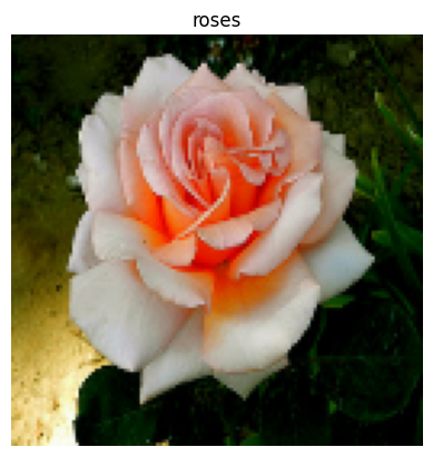
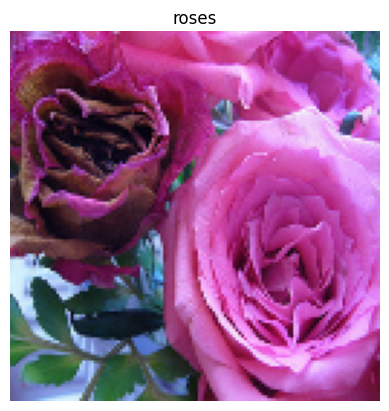
보다 현실적인 예를 보려면 preprocessing.image.ImageDataGenerator를 tf.data.Dataset로 래핑해 보세요.
먼저, 데이터를 다운로드합니다.
flowers = tf.keras.utils.get_file(
    'flower_photos',
    'https://storage.googleapis.com/download.tensorflow.org/example_images/flower_photos.tgz',
    untar=True)
Downloading data from https://storage.googleapis.com/download.tensorflow.org/example_images/flower_photos.tgz
228813984/228813984 [==============================] - 1s 0us/step
image.ImageDataGenerator를 만듭니다.
img_gen = tf.keras.preprocessing.image.ImageDataGenerator(rescale=1./255, rotation_range=20)
images, labels = next(img_gen.flow_from_directory(flowers))
Found 3670 images belonging to 5 classes.
print(images.dtype, images.shape)
print(labels.dtype, labels.shape)
float32 (32, 256, 256, 3)
float32 (32, 5)
ds = tf.data.Dataset.from_generator(
    lambda: img_gen.flow_from_directory(flowers),
    output_types=(tf.float32, tf.float32),
    output_shapes=([32,256,256,3], [32,5])
)

ds.element_spec
(TensorSpec(shape=(32, 256, 256, 3), dtype=tf.float32, name=None),
 TensorSpec(shape=(32, 5), dtype=tf.float32, name=None))
for images, labels in ds.take(1):
  print('images.shape: ', images.shape)
  print('labels.shape: ', labels.shape)
Found 3670 images belonging to 5 classes.
images.shape:  (32, 256, 256, 3)
labels.shape:  (32, 5)
TFRecord 데이터 소비하기
엔드 투 엔드 예제는 TFRecords 로드 튜토리얼을 참고하세요.
tf.data API는 다양한 파일 형식을 지원하므로 메모리에 맞지 않는 큰 데이터세트를 처리할 수 있습니다. 예를 들어, TFRecord 파일 형식은 많은 TensorFlow 애플리케이션이 학습 데이터에 사용하는 간단한 레코드 지향적 바이너리 형식입니다. tf.data.TFRecordDataset 클래스를 사용하면 입력 파이프라인의 일부로 하나 이상의 TFRecord 파일 내용을 스트리밍할 수 있습니다.
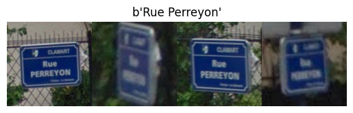
다음은 프랑스 도로명 표시(FSNS)의 테스트 파일을 사용한 예입니다.
# Creates a dataset that reads all of the examples from two files.
fsns_test_file = tf.keras.utils.get_file("fsns.tfrec", "https://storage.googleapis.com/download.tensorflow.org/data/fsns-20160927/testdata/fsns-00000-of-00001")
Downloading data from https://storage.googleapis.com/download.tensorflow.org/data/fsns-20160927/testdata/fsns-00000-of-00001
7904079/7904079 [==============================] - 0s 0us/step
TFRecordDataset 이니셜라이저(initializer)의 filenames 인수는 문자열, 문자열 목록 또는 tf.Tensor 문자열일 수 있습니다. 따라서 학습 및 검증 목적으로 두 파일 세트를 사용하는 경우, 파일 이름을 입력 인수로 사용하여 데이터세트를 생성하는 팩토리 메서드를 작성할 수 있습니다.
dataset = tf.data.TFRecordDataset(filenames = [fsns_test_file])
dataset
<TFRecordDatasetV2 element_spec=TensorSpec(shape=(), dtype=tf.string, name=None)>
많은 TensorFlow 프로젝트는 TFRecord 파일에서 직렬화된 tf.train.Example 레코드를 사용합니다. 검사하기 전에 이를 디코딩해야 합니다.
raw_example = next(iter(dataset))
parsed = tf.train.Example.FromString(raw_example.numpy())

parsed.features.feature['image/text']
bytes_list {
  value: "Rue Perreyon"
}
텍스트 데이터 소비하기
엔드 투 엔드 예제는 텍스트 로드 튜토리얼을 참고하세요.
많은 데이터세트가 하나 이상의 텍스트 파일로 배포됩니다. tf.data.TextLineDataset는 하나 이상의 텍스트 파일에서 줄을 추출하는 간편한 방법을 제공합니다. 하나 이상의 파일 이름이 주어지면 TextLineDataset는 이러한 파일의 줄당 하나의 문자열 값 요소를 생성합니다.
directory_url = 'https://storage.googleapis.com/download.tensorflow.org/data/illiad/'
file_names = ['cowper.txt', 'derby.txt', 'butler.txt']

file_paths = [
    tf.keras.utils.get_file(file_name, directory_url + file_name)
    for file_name in file_names
]
Downloading data from https://storage.googleapis.com/download.tensorflow.org/data/illiad/cowper.txt
815980/815980 [==============================] - 0s 0us/step
Downloading data from https://storage.googleapis.com/download.tensorflow.org/data/illiad/derby.txt
809730/809730 [==============================] - 0s 0us/step
Downloading data from https://storage.googleapis.com/download.tensorflow.org/data/illiad/butler.txt
807992/807992 [==============================] - 0s 0us/step
dataset = tf.data.TextLineDataset(file_paths)
첫 번째 파일의 처음 몇 줄은 다음과 같습니다.
for line in dataset.take(5):
  print(line.numpy())
b"\xef\xbb\xbfAchilles sing, O Goddess! Peleus' son;"
b'His wrath pernicious, who ten thousand woes'
b"Caused to Achaia's host, sent many a soul"
b'Illustrious into Ades premature,'
b'And Heroes gave (so stood the will of Jove)'
파일 사이에서 줄을 바꾸려면 Dataset.interleave를 사용합니다. 이렇게 하면 파일을 쉽게 섞을 수 있습니다. 각 변환의 첫 번째, 두 번째 및 세 번째 줄은 다음과 같습니다.
files_ds = tf.data.Dataset.from_tensor_slices(file_paths)
lines_ds = files_ds.interleave(tf.data.TextLineDataset, cycle_length=3)

for i, line in enumerate(lines_ds.take(9)):
  if i % 3 == 0:
    print()
  print(line.numpy())
b"\xef\xbb\xbfAchilles sing, O Goddess! Peleus' son;"
b"\xef\xbb\xbfOf Peleus' son, Achilles, sing, O Muse,"
b'\xef\xbb\xbfSing, O goddess, the anger of Achilles son of Peleus, that brought'

b'His wrath pernicious, who ten thousand woes'
b'The vengeance, deep and deadly; whence to Greece'
b'countless ills upon the Achaeans. Many a brave soul did it send'

b"Caused to Achaia's host, sent many a soul"
b'Unnumbered ills arose; which many a soul'
b'hurrying down to Hades, and many a hero did it yield a prey to dogs and'
기본적으로 TextLineDataset 은 각 파일의 모든 행을 생성하므로 파일이 헤더 행으로 시작하거나 주석이 포함 된 경우 바람직하지 않을 수 있습니다. 이러한 행은 Dataset.skip() 또는 Dataset.filter() 변환을 사용하여 제거 할 수 있습니다. 여기서 첫 번째 줄을 건너 뛰고 생존자를 찾기 위해 필터링합니다.
titanic_file = tf.keras.utils.get_file("train.csv", "https://storage.googleapis.com/tf-datasets/titanic/train.csv")
titanic_lines = tf.data.TextLineDataset(titanic_file)
for line in titanic_lines.take(10):
  print(line.numpy())
b'survived,sex,age,n_siblings_spouses,parch,fare,class,deck,embark_town,alone'
b'0,male,22.0,1,0,7.25,Third,unknown,Southampton,n'
b'1,female,38.0,1,0,71.2833,First,C,Cherbourg,n'
b'1,female,26.0,0,0,7.925,Third,unknown,Southampton,y'
b'1,female,35.0,1,0,53.1,First,C,Southampton,n'
b'0,male,28.0,0,0,8.4583,Third,unknown,Queenstown,y'
b'0,male,2.0,3,1,21.075,Third,unknown,Southampton,n'
b'1,female,27.0,0,2,11.1333,Third,unknown,Southampton,n'
b'1,female,14.0,1,0,30.0708,Second,unknown,Cherbourg,n'
b'1,female,4.0,1,1,16.7,Third,G,Southampton,n'
def survived(line):
  return tf.not_equal(tf.strings.substr(line, 0, 1), "0")

survivors = titanic_lines.skip(1).filter(survived)
for line in survivors.take(10):
  print(line.numpy())
b'1,female,38.0,1,0,71.2833,First,C,Cherbourg,n'
b'1,female,26.0,0,0,7.925,Third,unknown,Southampton,y'
b'1,female,35.0,1,0,53.1,First,C,Southampton,n'
b'1,female,27.0,0,2,11.1333,Third,unknown,Southampton,n'
b'1,female,14.0,1,0,30.0708,Second,unknown,Cherbourg,n'
b'1,female,4.0,1,1,16.7,Third,G,Southampton,n'
b'1,male,28.0,0,0,13.0,Second,unknown,Southampton,y'
b'1,female,28.0,0,0,7.225,Third,unknown,Cherbourg,y'
b'1,male,28.0,0,0,35.5,First,A,Southampton,y'
b'1,female,38.0,1,5,31.3875,Third,unknown,Southampton,n'
CSV 데이터 소비하기
자세한 예는 CSV 파일 로드 및 Pandas DataFrames 로드 튜토리얼을 참고하세요.
CSV 파일 형식은 표 형식의 데이터를 일반 텍스트로 저장하는 데 널리 이용되는 형식입니다.
예를 들면 다음과 같습니다.
titanic_file = tf.keras.utils.get_file("train.csv", "https://storage.googleapis.com/tf-datasets/titanic/train.csv")
df = pd.read_csv(titanic_file)
df.head()
데이터가 메모리에 맞는 경우 동일한 Dataset.from_tensor_slices 메서드가 사전에서 작동하여 이 데이터를 쉽게 가져올 수 있습니다.
titanic_slices = tf.data.Dataset.from_tensor_slices(dict(df))

for feature_batch in titanic_slices.take(1):
  for key, value in feature_batch.items():
    print("  {!r:20s}: {}".format(key, value))
'survived'          : 0
  'sex'               : b'male'
  'age'               : 22.0
  'n_siblings_spouses': 1
  'parch'             : 0
  'fare'              : 7.25
  'class'             : b'Third'
  'deck'              : b'unknown'
  'embark_town'       : b'Southampton'
  'alone'             : b'n'
보다 확장성 있는 접근 방식은 필요에 따라 디스크에서 로드하는 것입니다.
tf.data 모듈은 RFC 4180을 준수하는 하나 이상의 CSV 파일에서 레코드를 추출하는 메서드를 제공합니다.
tf.data.experimental.make_csv_dataset 함수는 csv 파일 세트를 읽기위한 고급 인터페이스입니다. 열 형식 유추와 일괄 처리 및 셔플링과 같은 많은 기능을 지원하며 사용이 간편합니다.
titanic_batches = tf.data.experimental.make_csv_dataset(
    titanic_file, batch_size=4,
    label_name="survived")
for feature_batch, label_batch in titanic_batches.take(1):
  print("'survived': {}".format(label_batch))
  print("features:")
  for key, value in feature_batch.items():
    print("  {!r:20s}: {}".format(key, value))
'survived': [0 0 1 0]
features:
  'sex'               : [b'male' b'male' b'female' b'male']
  'age'               : [17. 19. 28. 39.]
  'n_siblings_spouses': [1 0 0 0]
  'parch'             : [1 0 0 0]
  'fare'              : [ 7.2292  0.      7.225  24.15  ]
  'class'             : [b'Third' b'Third' b'Third' b'Third']
  'deck'              : [b'unknown' b'unknown' b'unknown' b'unknown']
  'embark_town'       : [b'Cherbourg' b'Southampton' b'Cherbourg' b'Southampton']
  'alone'             : [b'n' b'y' b'y' b'y']
열의 일부만 필요한 경우 select_columns 인수를 사용할 수 있습니다.
titanic_batches = tf.data.experimental.make_csv_dataset(
    titanic_file, batch_size=4,
    label_name="survived", select_columns=['class', 'fare', 'survived'])
for feature_batch, label_batch in titanic_batches.take(1):
  print("'survived': {}".format(label_batch))
  for key, value in feature_batch.items():
    print("  {!r:20s}: {}".format(key, value))
'survived': [1 0 1 0]
  'fare'              : [  7.775    7.65   133.65     7.3125]
  'class'             : [b'Third' b'Third' b'First' b'Third']
보다 세밀한 제어를 제공하는 하위 수준의 experimental.CsvDataset 클래스도 있습니다. 이 클래스는 열 형식 유추를 지원하지 않으며, 대신 각 열의 유형을 지정해야 합니다.
titanic_types  = [tf.int32, tf.string, tf.float32, tf.int32, tf.int32, tf.float32, tf.string, tf.string, tf.string, tf.string]
dataset = tf.data.experimental.CsvDataset(titanic_file, titanic_types , header=True)

for line in dataset.take(10):
  print([item.numpy() for item in line])
[0, b'male', 22.0, 1, 0, 7.25, b'Third', b'unknown', b'Southampton', b'n']
[1, b'female', 38.0, 1, 0, 71.2833, b'First', b'C', b'Cherbourg', b'n']
[1, b'female', 26.0, 0, 0, 7.925, b'Third', b'unknown', b'Southampton', b'y']
[1, b'female', 35.0, 1, 0, 53.1, b'First', b'C', b'Southampton', b'n']
[0, b'male', 28.0, 0, 0, 8.4583, b'Third', b'unknown', b'Queenstown', b'y']
[0, b'male', 2.0, 3, 1, 21.075, b'Third', b'unknown', b'Southampton', b'n']
[1, b'female', 27.0, 0, 2, 11.1333, b'Third', b'unknown', b'Southampton', b'n']
[1, b'female', 14.0, 1, 0, 30.0708, b'Second', b'unknown', b'Cherbourg', b'n']
[1, b'female', 4.0, 1, 1, 16.7, b'Third', b'G', b'Southampton', b'n']
[0, b'male', 20.0, 0, 0, 8.05, b'Third', b'unknown', b'Southampton', b'y']
일부 열이 비어있는 경우 이 낮은 수준의 인터페이스를 통해 열 유형 대신 기본값을 제공할 수 있습니다.
%%writefile missing.csv
1,2,3,4
,2,3,4
1,,3,4
1,2,,4
1,2,3,
,,,
Writing missing.csv
# Creates a dataset that reads all of the records from two CSV files, each with
# four float columns which may have missing values.

record_defaults = [999,999,999,999]
dataset = tf.data.experimental.CsvDataset("missing.csv", record_defaults)
dataset = dataset.map(lambda *items: tf.stack(items))
dataset
<MapDataset element_spec=TensorSpec(shape=(4,), dtype=tf.int32, name=None)>
for line in dataset:
  print(line.numpy())
[1 2 3 4]
[999   2   3   4]
[  1 999   3   4]
[  1   2 999   4]
[  1   2   3 999]
[999 999 999 999]
기본적으로, CsvDataset는 파일에 있는 모든 줄의 모든 열을 생성하기 때문에, 예를 들어 파일이 무시해야 하는 헤더 줄로 시작하거나 일부 열이 입력에 필요하지 않은 경우 바람직하지 않을 수 있습니다. 이러한 줄과 필드는 header 및 select_cols 인수로 제거할 수 있습니다.
# Creates a dataset that reads all of the records from two CSV files with
# headers, extracting float data from columns 2 and 4.
record_defaults = [999, 999] # Only provide defaults for the selected columns
dataset = tf.data.experimental.CsvDataset("missing.csv", record_defaults, select_cols=[1, 3])
dataset = dataset.map(lambda *items: tf.stack(items))
dataset
<MapDataset element_spec=TensorSpec(shape=(2,), dtype=tf.int32, name=None)>
for line in dataset:
  print(line.numpy())
[2 4]
[2 4]
[999   4]
[2 4]
[  2 999]
[999 999]
파일 세트 소비하기
파일 세트로 분배된 많은 데이터세트가 있으며, 여기서 각 파일은 예입니다.
flowers_root = tf.keras.utils.get_file(
    'flower_photos',
    'https://storage.googleapis.com/download.tensorflow.org/example_images/flower_photos.tgz',
    untar=True)
flowers_root = pathlib.Path(flowers_root)
참고: 이러한 이미지는 라이센스가 있는 CC-BY입니다. 자세한 내용은 LICENSE.txt를 참조하세요.
루트 디렉토리에는 각 클래스에 대한 디렉토리가 있습니다.
for item in flowers_root.glob("*"):
  print(item.name)
daisy
sunflowers
LICENSE.txt
dandelion
tulips
roses
각 클래스 디렉토리의 파일은 예입니다.
list_ds = tf.data.Dataset.list_files(str(flowers_root/'*/*'))

for f in list_ds.take(5):
  print(f.numpy())
b'/home/kbuilder/.keras/datasets/flower_photos/daisy/3720632920_93cf1cc7f3_m.jpg'
b'/home/kbuilder/.keras/datasets/flower_photos/daisy/5673551_01d1ea993e_n.jpg'
b'/home/kbuilder/.keras/datasets/flower_photos/dandelion/4528742654_99d233223b_m.jpg'
b'/home/kbuilder/.keras/datasets/flower_photos/sunflowers/9558630626_52a1b7d702_m.jpg'
b'/home/kbuilder/.keras/datasets/flower_photos/daisy/9299302012_958c70564c_n.jpg'
tf.io.read_file 함수를 사용하여 데이터를 읽고 경로에서 레이블을 추출하여 (image, label) 쌍을 반환합니다.
def process_path(file_path):
  label = tf.strings.split(file_path, os.sep)[-2]
  return tf.io.read_file(file_path), label

labeled_ds = list_ds.map(process_path)
for image_raw, label_text in labeled_ds.take(1):
  print(repr(image_raw.numpy()[:100]))
  print()
  print(label_text.numpy())
b'\xff\xd8\xff\xe0\x00\x10JFIF\x00\x01\x01\x00\x00\x01\x00\x01\x00\x00\xff\xdb\x00C\x00\x03\x02\x02\x03\x02\x02\x03\x03\x03\x03\x04\x03\x03\x04\x05\x08\x05\x05\x04\x04\x05\n\x07\x07\x06\x08\x0c\n\x0c\x0c\x0b\n\x0b\x0b\r\x0e\x12\x10\r\x0e\x11\x0e\x0b\x0b\x10\x16\x10\x11\x13\x14\x15\x15\x15\x0c\x0f\x17\x18\x16\x14\x18\x12\x14\x15\x14\xff\xdb\x00C\x01\x03\x04\x04\x05\x04\x05'

b'dandelion'
데이터세트 요소 배치 처리하기
간단한 배치 처리
가장 간단한 형태의 배치 처리는 데이터세트의 n 연속 요소를 단일 요소로 스태킹합니다. Dataset.batch() 변환은 요소의 각 구성 요소에 적용되는 tf.stack() 연산자와 동일한 제약 조건으로 정확하게 이 동작을 수행합니다. 즉, 각 구성 요소 i에서 모든 요소는 정확히 같은 형상의 텐서를 가져야 합니다.
inc_dataset = tf.data.Dataset.range(100)
dec_dataset = tf.data.Dataset.range(0, -100, -1)
dataset = tf.data.Dataset.zip((inc_dataset, dec_dataset))
batched_dataset = dataset.batch(4)

for batch in batched_dataset.take(4):
  print([arr.numpy() for arr in batch])
[array([0, 1, 2, 3]), array([ 0, -1, -2, -3])]
[array([4, 5, 6, 7]), array([-4, -5, -6, -7])]
[array([ 8,  9, 10, 11]), array([ -8,  -9, -10, -11])]
[array([12, 13, 14, 15]), array([-12, -13, -14, -15])]
tf.data가 형상 정보를 전파하려고 할 때 Dataset.batch의 기본 설정에서 알 수 없는 배치 크기가 생겨나는데, 마지막 배치가 완전히 채워지지 않았을 수 있기 때문입니다. 형상에서 None에 주목하세요.
batched_dataset
<BatchDataset element_spec=(TensorSpec(shape=(None,), dtype=tf.int64, name=None), TensorSpec(shape=(None,), dtype=tf.int64, name=None))>
drop_remainder 인수를 사용하여 이 마지막 배치를 무시하고 전체 형상 전파를 얻습니다.
batched_dataset = dataset.batch(7, drop_remainder=True)
batched_dataset
<BatchDataset element_spec=(TensorSpec(shape=(7,), dtype=tf.int64, name=None), TensorSpec(shape=(7,), dtype=tf.int64, name=None))>
패딩이 있는 텐서 배치 처리하기
위의 레시피는 모두 같은 크기의 텐서에 적용됩니다. 그러나 많은 모델(예: 시퀀스 모델)은 다양한 크기(예: 다른 길이의 시퀀스)를 가질 수 있는 입력 데이터로 작동합니다. 이러한 경우에 Dataset.padded_batch 변환을 사용하면 패딩 처리될 수 있는 하나 이상의 차원을 지정하여 서로 다른 형상의 텐서를 배치 처리할 수 있습니다.
dataset = tf.data.Dataset.range(100)
dataset = dataset.map(lambda x: tf.fill([tf.cast(x, tf.int32)], x))
dataset = dataset.padded_batch(4, padded_shapes=(None,))

for batch in dataset.take(2):
  print(batch.numpy())
  print()
[[0 0 0]
 [1 0 0]
 [2 2 0]
 [3 3 3]]

[[4 4 4 4 0 0 0]
 [5 5 5 5 5 0 0]
 [6 6 6 6 6 6 0]
 [7 7 7 7 7 7 7]]
Dataset.padded_batch 변환을 사용하면 각 구성 요소의 각 차원에 대해 서로 다른 패딩을 설정할 수 있으며, 이는 가변 길이(위 예제에서 None으로 표시됨) 또는 상수 길이일 수 있습니다. 기본값이 0인 패딩 값을 재정의할 수도 있습니다.
학습 워크플로우
여러 epoch 처리하기
tf.data API는 동일한 데이터의 여러 epoch를 처리하는 두 가지 주요 방법을 제공합니다.
여러 epoch에서 데이터세트를 반복하는 가장 간단한 방법은 Dataset.repeat() 변환을 사용하는 것입니다. 먼저 titanic 데이터의 데이터세트를 만듭니다.
titanic_file = tf.keras.utils.get_file("train.csv", "https://storage.googleapis.com/tf-datasets/titanic/train.csv")
titanic_lines = tf.data.TextLineDataset(titanic_file)
def plot_batch_sizes(ds):
  batch_sizes = [batch.shape[0] for batch in ds]
  plt.bar(range(len(batch_sizes)), batch_sizes)
  plt.xlabel('Batch number')
  plt.ylabel('Batch size')
인수 없이 Dataset.repeat() 변환을 적용하면 입력이 무한히 반복됩니다.
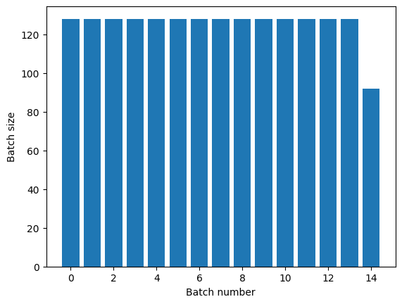
Dataset.repeat 변환은 한 epoch의 끝과 다음 epoch의 시작을 알리지 않고 인수를 연결합니다. 이 때문에 Dataset.batch 후에 적용된 Dataset.repeat는 epoch 경계 양쪽에 걸쳐진 배치를 생성합니다.
titanic_batches = titanic_lines.repeat(3).batch(128)
plot_batch_sizes(titanic_batches)
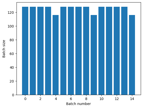
명확한 epoch 분리가 필요한 경우, 반복하기 전에 Dataset.batch를 넣으세요.
titanic_batches = titanic_lines.batch(128).repeat(3)

plot_batch_sizes(titanic_batches)
각 Epoch가 끝날 때 사용자 정의 계산(예: 통계 수집)을 수행하려면 각 Epoch에서 데이터세트 반복을 다시 시작하는 것이 가장 간단합니다.
epochs = 3
dataset = titanic_lines.batch(128)

for epoch in range(epochs):
  for batch in dataset:
    print(batch.shape)
  print("End of epoch: ", epoch)
(128,)
(128,)
(128,)
(128,)
(116,)
End of epoch:  0
(128,)
(128,)
(128,)
(128,)
(116,)
End of epoch:  1
(128,)
(128,)
(128,)
(128,)
(116,)
End of epoch:  2
입력 데이터의 임의 셔플
Dataset.shuffle() 변환은 고정 크기 버퍼를 유지하고 해당 버퍼에서 무작위로 다음 요소를 균일하게 선택합니다.
참고: 큰 buffer_sizes는 더 철저하게 셔플되지만 채우는 데 많은 메모리와 상당한 시간이 소요될 수 있습니다. 이것이 문제가 되는 경우 파일 전체에서 Dataset.interleave를 사용하세요.
효과를 확인할 수 있도록 데이터세트에 인덱스를 추가합니다.
lines = tf.data.TextLineDataset(titanic_file)
counter = tf.data.experimental.Counter()

dataset = tf.data.Dataset.zip((counter, lines))
dataset = dataset.shuffle(buffer_size=100)
dataset = dataset.batch(20)
dataset
WARNING:tensorflow:From /tmpfs/tmp/ipykernel_161777/4092668703.py:2: CounterV2 (from tensorflow.python.data.experimental.ops.counter) is deprecated and will be removed in a future version.
Instructions for updating:
Use `tf.data.Dataset.counter(...)` instead.
<BatchDataset element_spec=(TensorSpec(shape=(None,), dtype=tf.int64, name=None), TensorSpec(shape=(None,), dtype=tf.string, name=None))>
buffer_size가 100이고 배치 크기가 20이므로 첫 번째 배치에는 120 이상의 인덱스를 가진 요소가 없습니다.
n,line_batch = next(iter(dataset))
print(n.numpy())
[19 80 77 52 22 28 91 70 35 26 44 49 13 58 11 66 40 76 94 7]
Dataset.batch의 경우와 마찬가지로 Dataset.repeat에 상대적인 순서가 중요합니다.
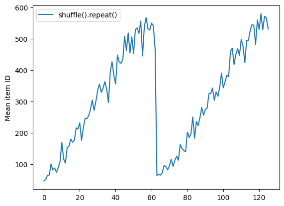
셔플 버퍼가 비워질 때까지 Dataset.shuffle은 epoch의 끝을 알리지 않습니다. 따라서 반복 전에 놓여진 셔플은 다음 epoch로 이동하기 전에 한 epoch의 모든 요소를 표시합니다.
dataset = tf.data.Dataset.zip((counter, lines))
shuffled = dataset.shuffle(buffer_size=100).batch(10).repeat(2)

print("Here are the item ID's near the epoch boundary:\n")
for n, line_batch in shuffled.skip(60).take(5):
  print(n.numpy())
Here are the item ID's near the epoch boundary:

[460 615 472 416 161 609 547 589 432 425]
[519 570 525 487 504 587 491 252 528 627]
[394 588 604 515 601 626 584 558]
[63 64 72 75 15 79 57 42 21 19]
[67 43 36  7 73  3 70 46 78 45]
shuffle_repeat = [n.numpy().mean() for n, line_batch in shuffled]
plt.plot(shuffle_repeat, label="shuffle().repeat()")
plt.ylabel("Mean item ID")
plt.legend()
<matplotlib.legend.Legend at 0x7ff5980f09d0>
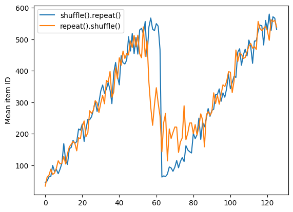
그러나 반복이 셔플 앞에 있으면 epoch 경계가 섞여버립니다.
dataset = tf.data.Dataset.zip((counter, lines))
shuffled = dataset.repeat(2).shuffle(buffer_size=100).batch(10)

print("Here are the item ID's near the epoch boundary:\n")
for n, line_batch in shuffled.skip(55).take(15):
  print(n.numpy())
Here are the item ID's near the epoch boundary:

[557 450 343 538 529  16 580   2 611 623]
[459 620   4 567 561 359 536  34 572 518]
[571  40 542  39  38 599 588 574 261 316]
[534 606 622  52 592  26  41 550 464 424]
[ 49 303 564 584 373   8 591  46  20 523]
[582 551 374 457 597  17  44  31  66  27]
[ 54   7 590  42  63 441 514 625 417 595]
[578 531  28  71 462  69  11  70  91  10]
[ 23  76  59 442   6  72   3 617 627 528]
[ 81 543 596  80  19  96  43 116  50  99]
[537  97 104  93   5  14  25 587 430 111]
[ 73 127  13  62  78  82 121 624 105 103]
[ 74  92 483  55  64 143  37 142 106  18]
[484 119  51 145 131 128  30  60  87 109]
[101 122  67 153 114  22  98  77 110   1]
repeat_shuffle = [n.numpy().mean() for n, line_batch in shuffled]

plt.plot(shuffle_repeat, label="shuffle().repeat()")
plt.plot(repeat_shuffle, label="repeat().shuffle()")
plt.ylabel("Mean item ID")
plt.legend()
<matplotlib.legend.Legend at 0x7ff598187190>
데이터 전처리하기
Dataset.map(f) 변환은 주어진 함수 f를 입력 데이터세트의 각 요소에 적용하여 새 데이터세트를 생성합니다. 여기서 함수형 프로그래밍 언어의 목록(및 기타 구조)에 일반적으로 적용되는 map() 함수가 그 기초를 이룹니다. 함수 f는 입력에서 단일 요소를 나타내는 tf.Tensor 객체를 가져와 새 데이터세트에서 단일 요소를 나타내는 tf.Tensor 객체를 반환합니다. 구현시 표준 TensorFlow 작업을 사용하여 한 요소를 다른 요소로 변환합니다.
이 섹션에서는 Dataset.map() 사용 방법에 대한 일반적인 예를 다룹니다.
이미지 데이터 디코딩 및 크기 조정하기
실제 이미지 데이터에서 신경망을 학습할 때 크기가 다른 이미지를 일반적 크기로 변환하여 고정 크기로 배치 처리될 수 있도록 해야 하는 경우가 종종 있습니다.
꽃 파일 이름 데이터세트를 다시 빌드합니다.
list_ds = tf.data.Dataset.list_files(str(flowers_root/'*/*'))
데이터세트 요소를 조작하는 함수를 작성합니다.
# Reads an image from a file, decodes it into a dense tensor, and resizes it
# to a fixed shape.
def parse_image(filename):
  parts = tf.strings.split(filename, os.sep)
  label = parts[-2]

  image = tf.io.read_file(filename)
  image = tf.io.decode_jpeg(image)
  image = tf.image.convert_image_dtype(image, tf.float32)
  image = tf.image.resize(image, [128, 128])
  return image, label
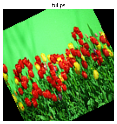
제대로 작동하는지 테스트합니다.
file_path = next(iter(list_ds))
image, label = parse_image(file_path)

def show(image, label):
  plt.figure()
  plt.imshow(image)
  plt.title(label.numpy().decode('utf-8'))
  plt.axis('off')

show(image, label)

데이터세트에 매핑합니다.
images_ds = list_ds.map(parse_image)

for image, label in images_ds.take(2):
  show(image, label)
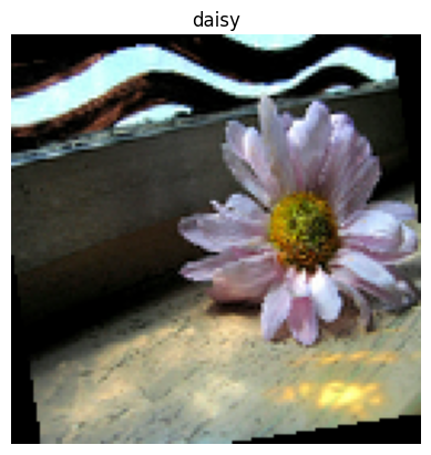
임의의 Python 로직 적용하기
성능상의 이유로 가능하면 데이터를 사전 처리하기 위해 TensorFlow 연산을 사용해야 합니다. 그러나 입력 데이터를 구문 분석할 때 외부 Python 라이브러리를 호출하는 것이 유용한 경우가 있습니다. Dataset.map 변환에서 tf.py_function 연산을 사용할 수 있습니다
예를 들어, 임의 회전을 적용하려는 경우 tf.image 모듈에는 tf.image.rot90만 있으므로 이미지 확대에는 그다지 유용하지 않습니다.
참고: tensorflow_addons에는 tensorflow_addons.image.rotate에 TensorFlow와 호환되는 rotate가 있습니다.
tf.py_function을 데모하려면 scipy.ndimage.rotate 함수를 대신 사용해보세요.
import scipy.ndimage as ndimage

def random_rotate_image(image):
  image = ndimage.rotate(image, np.random.uniform(-30, 30), reshape=False)
  return image
image, label = next(iter(images_ds))
image = random_rotate_image(image)
show(image, label)
Clipping input data to the valid range for imshow with RGB data ([0..1] for floats or [0..255] for integers).
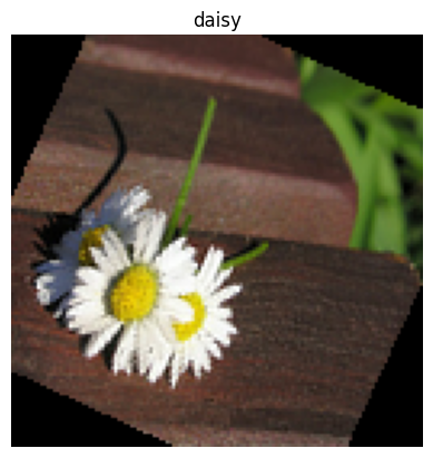
이 함수를 Dataset.map과 함께 사용하려면 Dataset.from_generator의 경우와 같은 주의 사항이 적용되는데, 함수를 적용할 때 반환 형상과 유형을 설명해야 합니다.
def tf_random_rotate_image(image, label):
  im_shape = image.shape
  [image,] = tf.py_function(random_rotate_image, [image], [tf.float32])
  image.set_shape(im_shape)
  return image, label
rot_ds = images_ds.map(tf_random_rotate_image)

for image, label in rot_ds.take(2):
  show(image, label)
Clipping input data to the valid range for imshow with RGB data ([0..1] for floats or [0..255] for integers).
Clipping input data to the valid range for imshow with RGB data ([0..1] for floats or [0..255] for integers).
tf.Example 프로토콜 버퍼 메시지 구문 분석하기
많은 입력 파이프라인이 TFRecord 형식에서 tf.train.Example 프로토콜 버퍼 메시지를 추출합니다. 각 tf.train.Example 레코드에는 하나 이상의 "기능"이 포함되며 입력 파이프라인은 일반적으로 이러한 기능을 텐서로 변환합니다.
fsns_test_file = tf.keras.utils.get_file("fsns.tfrec", "https://storage.googleapis.com/download.tensorflow.org/data/fsns-20160927/testdata/fsns-00000-of-00001")
dataset = tf.data.TFRecordDataset(filenames = [fsns_test_file])
dataset
<TFRecordDatasetV2 element_spec=TensorSpec(shape=(), dtype=tf.string, name=None)>
데이터를 이해하기 위해 tf.data.Dataset 외부에서 tf.train.Example 프로토콜로 작업할 수 있습니다.
raw_example = next(iter(dataset))
parsed = tf.train.Example.FromString(raw_example.numpy())

feature = parsed.features.feature
raw_img = feature['image/encoded'].bytes_list.value[0]
img = tf.image.decode_png(raw_img)
plt.imshow(img)
plt.axis('off')
_ = plt.title(feature["image/text"].bytes_list.value[0])
raw_example = next(iter(dataset))
def tf_parse(eg):
  example = tf.io.parse_example(
      eg[tf.newaxis], {
          'image/encoded': tf.io.FixedLenFeature(shape=(), dtype=tf.string),
          'image/text': tf.io.FixedLenFeature(shape=(), dtype=tf.string)
      })
  return example['image/encoded'][0], example['image/text'][0]
img, txt = tf_parse(raw_example)
print(txt.numpy())
print(repr(img.numpy()[:20]), "...")
b'Rue Perreyon'
b'\x89PNG\r\n\x1a\n\x00\x00\x00\rIHDR\x00\x00\x02X' ...
decoded = dataset.map(tf_parse)
decoded
<MapDataset element_spec=(TensorSpec(shape=(), dtype=tf.string, name=None), TensorSpec(shape=(), dtype=tf.string, name=None))>
image_batch, text_batch = next(iter(decoded.batch(10)))
image_batch.shape
TensorShape([10])
시계열 윈도잉
엔드 투 엔드 시계열 예시는 시계열 예측을 참고하십시오.
시계열 데이터는 시간 축을 그대로 유지하여 구성되는 경우가 많습니다.
간단한 Dataset.range를 사용하여 데모해 보겠습니다.
range_ds = tf.data.Dataset.range(100000)
일반적으로, 이러한 종류의 데이터를 기반으로 하는 모델에는 인접한 시간 조각이 필요할 것입니다.
가장 간단한 방법은 데이터를 배치 처리하는 것입니다.
batch 사용하기
batches = range_ds.batch(10, drop_remainder=True)

for batch in batches.take(5):
  print(batch.numpy())
[0 1 2 3 4 5 6 7 8 9]
[10 11 12 13 14 15 16 17 18 19]
[20 21 22 23 24 25 26 27 28 29]
[30 31 32 33 34 35 36 37 38 39]
[40 41 42 43 44 45 46 47 48 49]
또는 한 단계 미례로 들어간 밀집된 예측을 하려면 기능과 레이블을 서로 상대적으로 한 단계씩 이동시킬 수 있습니다.
def dense_1_step(batch):
  # Shift features and labels one step relative to each other.
  return batch[:-1], batch[1:]

predict_dense_1_step = batches.map(dense_1_step)

for features, label in predict_dense_1_step.take(3):
  print(features.numpy(), " => ", label.numpy())
[0 1 2 3 4 5 6 7 8]  =>  [1 2 3 4 5 6 7 8 9]
[10 11 12 13 14 15 16 17 18]  =>  [11 12 13 14 15 16 17 18 19]
[20 21 22 23 24 25 26 27 28]  =>  [21 22 23 24 25 26 27 28 29]
고정 오프셋 대신 전체 윈도우를 예측하려면 배치를 두 부분으로 분할할 수 있습니다.
batches = range_ds.batch(15, drop_remainder=True)

def label_next_5_steps(batch):
  return (batch[:-5],   # Inputs: All except the last 5 steps
          batch[-5:])   # Labels: The last 5 steps

predict_5_steps = batches.map(label_next_5_steps)

for features, label in predict_5_steps.take(3):
  print(features.numpy(), " => ", label.numpy())
[0 1 2 3 4 5 6 7 8 9]  =>  [10 11 12 13 14]
[15 16 17 18 19 20 21 22 23 24]  =>  [25 26 27 28 29]
[30 31 32 33 34 35 36 37 38 39]  =>  [40 41 42 43 44]
한 배치의 기능과 다른 배치의 레이블이 약간 겹치게 하려면 Dataset.zip을 사용하세요.
feature_length = 10
label_length = 3

features = range_ds.batch(feature_length, drop_remainder=True)
labels = range_ds.batch(feature_length).skip(1).map(lambda labels: labels[:label_length])

predicted_steps = tf.data.Dataset.zip((features, labels))

for features, label in predicted_steps.take(5):
  print(features.numpy(), " => ", label.numpy())
[0 1 2 3 4 5 6 7 8 9]  =>  [10 11 12]
[10 11 12 13 14 15 16 17 18 19]  =>  [20 21 22]
[20 21 22 23 24 25 26 27 28 29]  =>  [30 31 32]
[30 31 32 33 34 35 36 37 38 39]  =>  [40 41 42]
[40 41 42 43 44 45 46 47 48 49]  =>  [50 51 52]
window 사용하기
Dataset.batch를 사용하는 동안 더 세밀한 제어가 필요한 상황이 있습니다. Dataset.window 메서드는 완전한 제어를 제공하지만 약간의 주의가 필요합니다. Datasets의 Dataset를 반환합니다. 자세한 내용은 데이터세트 구조를 참조하십시오.
window_size = 5

windows = range_ds.window(window_size, shift=1)
for sub_ds in windows.take(5):
  print(sub_ds)
<_VariantDataset element_spec=TensorSpec(shape=(), dtype=tf.int64, name=None)>
<_VariantDataset element_spec=TensorSpec(shape=(), dtype=tf.int64, name=None)>
<_VariantDataset element_spec=TensorSpec(shape=(), dtype=tf.int64, name=None)>
<_VariantDataset element_spec=TensorSpec(shape=(), dtype=tf.int64, name=None)>
<_VariantDataset element_spec=TensorSpec(shape=(), dtype=tf.int64, name=None)>
Dataset.flat_map 메서드는 데이터세트의 데이터세트를 가져와 단일 데이터세트로 병합할 수 있습니다.
for x in windows.flat_map(lambda x: x).take(30):
   print(x.numpy(), end=' ')
0 1 2 3 4 1 2 3 4 5 2 3 4 5 6 3 4 5 6 7 4 5 6 7 8 5 6 7 8 9
거의 모든 경우에 데이터세트를 먼저 Dataset.batch하게 될 것입니다.
def sub_to_batch(sub):
  return sub.batch(window_size, drop_remainder=True)

for example in windows.flat_map(sub_to_batch).take(5):
  print(example.numpy())
[0 1 2 3 4]
[1 2 3 4 5]
[2 3 4 5 6]
[3 4 5 6 7]
[4 5 6 7 8]
이제 shift 인수에 의해 각 윈도우가 이동하는 정도가 제어되는 것을 알 수 있습니다.
이것을 합치면 다음 함수를 작성할 수 있습니다.
def make_window_dataset(ds, window_size=5, shift=1, stride=1):
  windows = ds.window(window_size, shift=shift, stride=stride)

  def sub_to_batch(sub):
    return sub.batch(window_size, drop_remainder=True)

  windows = windows.flat_map(sub_to_batch)
  return windows
ds = make_window_dataset(range_ds, window_size=10, shift = 5, stride=3)

for example in ds.take(10):
  print(example.numpy())
[ 0  3  6  9 12 15 18 21 24 27]
[ 5  8 11 14 17 20 23 26 29 32]
[10 13 16 19 22 25 28 31 34 37]
[15 18 21 24 27 30 33 36 39 42]
[20 23 26 29 32 35 38 41 44 47]
[25 28 31 34 37 40 43 46 49 52]
[30 33 36 39 42 45 48 51 54 57]
[35 38 41 44 47 50 53 56 59 62]
[40 43 46 49 52 55 58 61 64 67]
[45 48 51 54 57 60 63 66 69 72]
그러면 이전과 같이 레이블을 쉽게 추출할 수 있습니다.
dense_labels_ds = ds.map(dense_1_step)

for inputs,labels in dense_labels_ds.take(3):
  print(inputs.numpy(), "=>", labels.numpy())
[ 0  3  6  9 12 15 18 21 24] => [ 3  6  9 12 15 18 21 24 27]
[ 5  8 11 14 17 20 23 26 29] => [ 8 11 14 17 20 23 26 29 32]
[10 13 16 19 22 25 28 31 34] => [13 16 19 22 25 28 31 34 37]
리샘플링
클래스 불균형이 매우 높은 데이터세트로 작업할 때는 데이터세트를 다시 샘플링해야 할 수 있습니다. tf.data는 이를 수행하기 위한 두 가지 방법을 제공합니다. 신용카드 사기 데이터세트가 이러한 종류의 문제를 보여주는 좋은 예입니다.
참고: 전체 튜토리얼을 보려면 불균형 데이터 분류로 이동하십시오.
zip_path = tf.keras.utils.get_file(
    origin='https://storage.googleapis.com/download.tensorflow.org/data/creditcard.zip',
    fname='creditcard.zip',
    extract=True)

csv_path = zip_path.replace('.zip', '.csv')
Downloading data from https://storage.googleapis.com/download.tensorflow.org/data/creditcard.zip
69155632/69155632 [==============================] - 0s 0us/step
creditcard_ds = tf.data.experimental.make_csv_dataset(
    csv_path, batch_size=1024, label_name="Class",
    # Set the column types: 30 floats and an int.
    column_defaults=[float()]*30+[int()])
이제 클래스의 분포를 확인해 보면 심하게 치우쳐져 있습니다.
def count(counts, batch):
  features, labels = batch
  class_1 = labels == 1
  class_1 = tf.cast(class_1, tf.int32)

  class_0 = labels == 0
  class_0 = tf.cast(class_0, tf.int32)

  counts['class_0'] += tf.reduce_sum(class_0)
  counts['class_1'] += tf.reduce_sum(class_1)

  return counts
counts = creditcard_ds.take(10).reduce(
    initial_state={'class_0': 0, 'class_1': 0},
    reduce_func = count)

counts = np.array([counts['class_0'].numpy(),
                   counts['class_1'].numpy()]).astype(np.float32)

fractions = counts/counts.sum()
print(fractions)
[0.9952 0.0048]
불균형 데이터세트를 사용하여 학습할 때의 일반적인 접근 방식은 균형을 맞추는 것입니다. tf.data에는 이 워크플로우를 가능하게 하는 몇 가지 메서드가 있습니다.
데이터세트 샘플링
데이터세트를 다시 샘플링하는 한 가지 방법은 sample_from_datasets를 사용하는 것입니다. 이는 각 클래스에 별도의 tf.data.Dataset가 있는 경우에 더 적합합니다.
여기서는 필터를 사용하여 신용카드 사기 데이터로부터 이를 생성합니다.
negative_ds = (
  creditcard_ds
    .unbatch()
    .filter(lambda features, label: label==0)
    .repeat())
positive_ds = (
  creditcard_ds
    .unbatch()
    .filter(lambda features, label: label==1)
    .repeat())
for features, label in positive_ds.batch(10).take(1):
  print(label.numpy())
[1 1 1 1 1 1 1 1 1 1]
tf.data.Dataset.sample_from_datasets를 사용하려면 데이터 세트와 각 가중치를 전달하십시오.
balanced_ds = tf.data.Dataset.sample_from_datasets(
    [negative_ds, positive_ds], [0.5, 0.5]).batch(10)
이제 데이터세트는 50/50 확률로 각 클래스의 예를 생성합니다.
for features, labels in balanced_ds.take(10):
  print(labels.numpy())
[1 1 0 0 0 0 0 0 1 0]
[1 1 0 1 1 1 1 0 1 0]
[0 0 1 0 1 1 1 1 1 1]
[1 1 0 0 0 1 1 0 0 1]
[0 0 0 0 0 0 1 1 0 1]
[1 0 1 1 0 0 1 1 0 1]
[0 1 1 1 1 1 0 0 0 0]
[1 1 1 0 1 1 1 0 0 0]
[1 0 1 0 1 0 0 1 1 0]
[0 0 0 0 1 1 0 1 0 0]
거부 리샘플링
위의 Dataset.sample_from_datasets 방식에서 한 가지 문제는 클래스별로 개별 tf.data.Dataset가 필요하다는 것입니다. Dataset.filter를 사용하면 되지만 그 결과로 모든 데이터가 두 번 로드됩니다.
tf.data.Dataset.rejection_resample 메서드는 한 번만 로드하여도 데이터세트에 적용하고 재조정할 수 있습니다. 균형을 이루기 위해 요소는 삭제되거나 반복됩니다.
rejection_resample 메서드는 class_func 인수를 사용합니다. 이 class_func는 각 데이터세트 요소에 적용되며 밸런싱을 위해 예제가 속한 클래스를 결정하는 데 사용됩니다.
여기의 목표는 레이블 분포의 균형을 맞추는 것이며 creditcard_ds의 요소는 이미 (features, label) 쌍입니다. 따라서 class_func 해당 레이블을 반환하면됩니다.
def class_func(features, label):
  return label
리샘플링 메서드는 개별 예제를 다루므로 이 메서드를 적용하기 전에 데이터세트를 unbatch 처리해야 합니다.
이 메서드는 대상 분포와 선택적으로 초기 분포 추정이 필요합니다.
resample_ds = (
    creditcard_ds
    .unbatch()
    .rejection_resample(class_func, target_dist=[0.5,0.5],
                        initial_dist=fractions)
    .batch(10))
WARNING:tensorflow:From /tmpfs/src/tf_docs_env/lib/python3.9/site-packages/tensorflow/python/data/ops/dataset_ops.py:6041: Print (from tensorflow.python.ops.logging_ops) is deprecated and will be removed after 2018-08-20.
Instructions for updating:
Use tf.print instead of tf.Print. Note that tf.print returns a no-output operator that directly prints the output. Outside of defuns or eager mode, this operator will not be executed unless it is directly specified in session.run or used as a control dependency for other operators. This is only a concern in graph mode. Below is an example of how to ensure tf.print executes in graph mode:
rejection_resample 메서드는 class가 class_func의 출력인 (class, example) 쌍을 반환합니다. 이 경우 example이 이미 (feature, label) 쌍이었으므로 map을 사용하여 레이블의 추가 복사본을 제거합니다.
balanced_ds = resample_ds.map(lambda extra_label, features_and_label: features_and_label)
이제 데이터세트는 50/50 확률로 각 클래스의 예를 생성합니다.
for features, labels in balanced_ds.take(10):
  print(labels.numpy())
Proportion of examples rejected by sampler is high: [0.99521482][0.99521482 0.00478515634][0 1]
Proportion of examples rejected by sampler is high: [0.99521482][0.99521482 0.00478515634][0 1]
Proportion of examples rejected by sampler is high: [0.99521482][0.99521482 0.00478515634][0 1]
Proportion of examples rejected by sampler is high: [0.99521482][0.99521482 0.00478515634][0 1]
Proportion of examples rejected by sampler is high: [0.99521482][0.99521482 0.00478515634][0 1]
Proportion of examples rejected by sampler is high: [0.99521482][0.99521482 0.00478515634][0 1]
Proportion of examples rejected by sampler is high: [0.99521482][0.99521482 0.00478515634][0 1]
Proportion of examples rejected by sampler is high: [0.99521482][0.99521482 0.00478515634][0 1]
Proportion of examples rejected by sampler is high: [0.99521482][0.99521482 0.00478515634][0 1]
Proportion of examples rejected by sampler is high: [0.99521482][0.99521482 0.00478515634][0 1]
[0 0 1 0 1 1 0 1 1 0]
[0 0 0 1 1 0 1 1 1 1]
[1 1 1 1 0 1 0 1 1 0]
[1 0 1 0 1 0 0 1 1 0]
[1 1 1 0 1 1 1 0 0 1]
[1 1 1 0 1 1 1 0 1 0]
[1 0 1 1 0 1 1 1 0 1]
[0 0 0 0 0 0 1 0 1 1]
[0 0 0 1 1 0 0 0 0 1]
[0 1 0 0 1 1 1 1 1 1]
반복기 검사점 처리
Tensorflow는 체크 포인트를 지원하므로 교육 프로세스가 다시 시작될 때 최신 체크 포인트를 복원하여 대부분의 진행 상황을 복구 할 수 있습니다. 모델 변수를 체크 포인트하는 것 외에도 데이터 세트 반복기의 진행 상태를 체크 포인트할 수 있습니다. 이 방법은 큰 데이터세트가 있고 다시 시작할 때마다 데이터세트를 시작하지 않으려는 경우에 유용할 수 있습니다. 그러나 Dataset.shuffle 및 Dataset.prefetch와 같은 변환은 반복기 내의 버퍼링 요소를 필요로 하므로 반복기 체크 포인트가 클 수 있습니다.
검사점에 반복기를 포함시키려면 반복기를 tf.train.Checkpoint 생성자로 전달합니다.
range_ds = tf.data.Dataset.range(20)

iterator = iter(range_ds)
ckpt = tf.train.Checkpoint(step=tf.Variable(0), iterator=iterator)
manager = tf.train.CheckpointManager(ckpt, '/tmp/my_ckpt', max_to_keep=3)

print([next(iterator).numpy() for _ in range(5)])

save_path = manager.save()

print([next(iterator).numpy() for _ in range(5)])

ckpt.restore(manager.latest_checkpoint)

print([next(iterator).numpy() for _ in range(5)])
[0, 1, 2, 3, 4]
[5, 6, 7, 8, 9]
[5, 6, 7, 8, 9]
참고: tf.py_function와 같은 외부 상태에 의존하는 반복기는 체크포인트할 수 없습니다. 그렇게 하려고 하면 외부 상태에 대해 불편해하는 예외가 발생합니다.
tf.data with tf.keras 사용하기
tf.keras API는 머신러닝 모델 생성 및 실행의 많은 측면을 단순화합니다. Model.fit, Model.evaluate, Model.predict API는 데이터세트를 입력으로 지원합니다. 다음은 빠른 데이터세트 및 모델 설정입니다.
train, test = tf.keras.datasets.fashion_mnist.load_data()

images, labels = train
images = images/255.0
labels = labels.astype(np.int32)
fmnist_train_ds = tf.data.Dataset.from_tensor_slices((images, labels))
fmnist_train_ds = fmnist_train_ds.shuffle(5000).batch(32)

model = tf.keras.Sequential([
  tf.keras.layers.Flatten(),
  tf.keras.layers.Dense(10)
])

model.compile(optimizer='adam',
              loss=tf.keras.losses.SparseCategoricalCrossentropy(from_logits=True),
              metrics=['accuracy'])
Model.fit 및 Model.evaluate에 대해 필요한 작업은 (feature, label) 쌍의 데이터세트를 전달하는 것뿐입니다.
model.fit(fmnist_train_ds, epochs=2)
Epoch 1/2
1875/1875 [==============================] - 5s 2ms/step - loss: 0.6008 - accuracy: 0.7963
Epoch 2/2
1875/1875 [==============================] - 4s 2ms/step - loss: 0.4620 - accuracy: 0.8418
<keras.callbacks.History at 0x7ff62108b400>
예를 들어 Dataset.repeat를 호출하여 무한한 데이터세트를 전달하는 경우 steps_per_epoch 인수도 전달하면 됩니다.
model.fit(fmnist_train_ds.repeat(), epochs=2, steps_per_epoch=20)
Epoch 1/2
20/20 [==============================] - 0s 2ms/step - loss: 0.4966 - accuracy: 0.8359
Epoch 2/2
20/20 [==============================] - 0s 2ms/step - loss: 0.4751 - accuracy: 0.8344
<keras.callbacks.History at 0x7ff5907c56d0>
평가를 위해서는 평가 단계의 수를 전달할 수 있습니다.
loss, accuracy = model.evaluate(fmnist_train_ds)
print("Loss :", loss)
print("Accuracy :", accuracy)
1875/1875 [==============================] - 3s 2ms/step - loss: 0.4436 - accuracy: 0.8472
Loss : 0.4436156153678894
Accuracy : 0.8471500277519226
긴 데이터세트의 경우 평가할 단계 수를 설정합니다.
loss, accuracy = model.evaluate(fmnist_train_ds.repeat(), steps=10)
print("Loss :", loss)
print("Accuracy :", accuracy)
10/10 [==============================] - 0s 2ms/step - loss: 0.4113 - accuracy: 0.8594
Loss : 0.4113312363624573
Accuracy : 0.859375
Model.predict를 호출할 경우에는 레이블이 필요하지 않습니다.
predict_ds = tf.data.Dataset.from_tensor_slices(images).batch(32)
result = model.predict(predict_ds, steps = 10)
print(result.shape)
10/10 [==============================] - 0s 1ms/step
(320, 10)
그러나 레이블이 포함된 데이터세트를 전달하면 레이블이 무시됩니다.
result = model.predict(fmnist_train_ds, steps = 10)
print(result.shape)
10/10 [==============================] - 0s 1ms/step
(320, 10)