
| |
|
 GitHub でソースを表示 GitHub でソースを表示 |
|
セットアップ
import numpy as np
import tensorflow as tf
from tensorflow import keras
from tensorflow.keras import layers
2024-01-11 19:55:31.403237: E external/local_xla/xla/stream_executor/cuda/cuda_dnn.cc:9261] Unable to register cuDNN factory: Attempting to register factory for plugin cuDNN when one has already been registered
2024-01-11 19:55:31.403283: E external/local_xla/xla/stream_executor/cuda/cuda_fft.cc:607] Unable to register cuFFT factory: Attempting to register factory for plugin cuFFT when one has already been registered
2024-01-11 19:55:31.404886: E external/local_xla/xla/stream_executor/cuda/cuda_blas.cc:1515] Unable to register cuBLAS factory: Attempting to register factory for plugin cuBLAS when one has already been registered
前書き
Keras Functional API は、tf.keras.Sequential API よりも柔軟なモデルの作成が可能で、非線形トポロジー、共有レイヤー、さらには複数の入力または出力を持つモデル処理することができます。
これは、ディープラーニングのモデルは通常、レイヤーの有向非巡回グラフ(DAG)であるという考えに基づいてます。要するに、Functional API はレイヤーのグラフを構築する方法です。
次のモデルを考察してみましょう。
(input: 784-dimensional vectors)
       ↧
[Dense (64 units, relu activation)]
       ↧
[Dense (64 units, relu activation)]
       ↧
[Dense (10 units, softmax activation)]
       ↧
(output: logits of a probability distribution over 10 classes)
これは 3つ のレイヤーを持つ単純なグラフです。Functional API を使用してモデルを構築するために、まずは入力ノードを作成することから始めます。
inputs = keras.Input(shape=(784,))
データの形状は、784次元のベクトルとして設定されます。各サンプルの形状のみを指定するため、バッチサイズは常に省略されます。
例えば、(32, 32, 3)という形状の画像入力がある場合には、次を使用します。
# Just for demonstration purposes.
img_inputs = keras.Input(shape=(32, 32, 3))
返されるinputsには、モデルに供給する入力データの形状とdtypeについての情報を含みます。形状は次のとおりです。
inputs.shape
TensorShape([None, 784])
dtype は次のとおりです。
inputs.dtype
tf.float32
このinputsオブジェクトのレイヤーを呼び出して、レイヤーのグラフに新しいノードを作成します。
dense = layers.Dense(64, activation="relu")
x = dense(inputs)
「レイヤー呼び出し」アクションは、「入力」から作成したこのレイヤーまで矢印を描くようなものです。denseレイヤーに入力を「渡して」、xを取得します。
レイヤーのグラフにあと少しレイヤーを追加してみましょう。
x = layers.Dense(64, activation="relu")(x)
outputs = layers.Dense(10)(x)
この時点で、レイヤーのグラフの入力と出力を指定することにより、Modelを作成できます。
model = keras.Model(inputs=inputs, outputs=outputs, name="mnist_model")
モデルの概要がどのようなものか、確認しましょう。
model.summary()
Model: "mnist_model"
_________________________________________________________________
 Layer (type)                Output Shape              Param #
=================================================================
 input_1 (InputLayer)        [(None, 784)]             0

 dense (Dense)               (None, 64)                50240

 dense_1 (Dense)             (None, 64)                4160

 dense_2 (Dense)             (None, 10)                650

=================================================================
Total params: 55050 (215.04 KB)
Trainable params: 55050 (215.04 KB)
Non-trainable params: 0 (0.00 Byte)
_________________________________________________________________
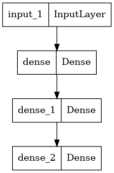
また、モデルをグラフとしてプロットすることも可能です。
keras.utils.plot_model(model, "my_first_model.png")
そしてオプションで、プロットされたグラフに各レイヤーの入力形状と出力形状を表示します 。
keras.utils.plot_model(model, "my_first_model_with_shape_info.png", show_shapes=True)
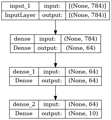
この図とコードはほぼ同じです。コードバージョンでは、接続矢印は呼び出し演算に置き換えられています。
「レイヤーのグラフ」はディープラーニングモデルの直感的なメンタルイメージであり、Functional API はこのメンタルイメージを忠実に映すモデルを作成する方法です。
トレーニング、評価、推論
Functional API を使用して構築されたモデルの学習、評価、推論は、Sequentialモデルの場合とまったく同じように動作します。
Model クラスにはトレーニングループ(fit() メソッド)と評価ループ(evaluate() メソッド)が組み込まれています。これらのループをカスタマイズすることで、教師あり学習を超えるトレーニングのルーチン(GAN など)を簡単に実装することができます。
ここでは、MNIST 画像データを読み込み、ベクトルに再形成し、(検証分割のパフォーマンスを監視しながら)データ上でモデルを当てはめ、その後、テストデータ上でモデルを評価します。
(x_train, y_train), (x_test, y_test) = keras.datasets.mnist.load_data()

x_train = x_train.reshape(60000, 784).astype("float32") / 255
x_test = x_test.reshape(10000, 784).astype("float32") / 255

model.compile(
    loss=keras.losses.SparseCategoricalCrossentropy(from_logits=True),
    optimizer=keras.optimizers.RMSprop(),
    metrics=["accuracy"],
)

history = model.fit(x_train, y_train, batch_size=64, epochs=2, validation_split=0.2)

test_scores = model.evaluate(x_test, y_test, verbose=2)
print("Test loss:", test_scores[0])
print("Test accuracy:", test_scores[1])
Epoch 1/2
WARNING: All log messages before absl::InitializeLog() is called are written to STDERR
I0000 00:00:1705002937.522982  228716 device_compiler.h:186] Compiled cluster using XLA!  This line is logged at most once for the lifetime of the process.
750/750 [==============================] - 3s 3ms/step - loss: 0.3431 - accuracy: 0.9034 - val_loss: 0.1855 - val_accuracy: 0.9453
Epoch 2/2
750/750 [==============================] - 2s 3ms/step - loss: 0.1553 - accuracy: 0.9548 - val_loss: 0.1380 - val_accuracy: 0.9601
313/313 - 0s - loss: 0.1356 - accuracy: 0.9592 - 489ms/epoch - 2ms/step
Test loss: 0.1356341540813446
Test accuracy: 0.9592000246047974
さらに詳しくはトレーニングと評価ガイドをご覧ください。
保存とシリアライズ
Functional API を使用して構築されたモデルの保存とシリアル化は、Sequentialのモデルと同じように動作します。Functional モデルを保存する標準的な方法は、model.save()を呼び出して、モデル全体を単一のファイルとして保存します。モデルを作成したコードが使用できなくなったとしても、後でこのファイルから同じモデルを再作成することが可能です。
保存されたファイルには次を含みます。
- モデルのアーキテクチャ
- モデルの重み値(トレーニングの間に学習された値)
- ある場合は、モデルトレーニング構成(
compileに渡される構成) - あれば、オプティマイザとその状態(中断した所からトレーニングを再開するため)
model.save("path_to_my_model")
del model
# Recreate the exact same model purely from the file:
model = keras.models.load_model("path_to_my_model")
INFO:tensorflow:Assets written to: path_to_my_model/assets
INFO:tensorflow:Assets written to: path_to_my_model/assets
詳細は、モデルシリアライゼーションと保存ガイドをご覧ください。
レイヤー群の同じグラフを使用してマルチモデルを定義する
Functional API では、モデルはレイヤー群のグラフでそれらの出入力を指定することにより生成されます。それはレイヤー群の単一のグラフ が複数のモデルを生成するために使用できることを意味しています。
次の例では、レイヤー群の同じスタックを使用して 2 つのモデルのインスタンス化を行います。これらは画像入力を 16 次元ベクトルに変換するencoderモデルと、トレーニングのためのエンドツーエンドautoencoderモデルです。
encoder_input = keras.Input(shape=(28, 28, 1), name="img")
x = layers.Conv2D(16, 3, activation="relu")(encoder_input)
x = layers.Conv2D(32, 3, activation="relu")(x)
x = layers.MaxPooling2D(3)(x)
x = layers.Conv2D(32, 3, activation="relu")(x)
x = layers.Conv2D(16, 3, activation="relu")(x)
encoder_output = layers.GlobalMaxPooling2D()(x)

encoder = keras.Model(encoder_input, encoder_output, name="encoder")
encoder.summary()

x = layers.Reshape((4, 4, 1))(encoder_output)
x = layers.Conv2DTranspose(16, 3, activation="relu")(x)
x = layers.Conv2DTranspose(32, 3, activation="relu")(x)
x = layers.UpSampling2D(3)(x)
x = layers.Conv2DTranspose(16, 3, activation="relu")(x)
decoder_output = layers.Conv2DTranspose(1, 3, activation="relu")(x)

autoencoder = keras.Model(encoder_input, decoder_output, name="autoencoder")
autoencoder.summary()
Model: "encoder"
_________________________________________________________________
 Layer (type)                Output Shape              Param #
=================================================================
 img (InputLayer)            [(None, 28, 28, 1)]       0

 conv2d (Conv2D)             (None, 26, 26, 16)        160

 conv2d_1 (Conv2D)           (None, 24, 24, 32)        4640

 max_pooling2d (MaxPooling2  (None, 8, 8, 32)          0
 D)

 conv2d_2 (Conv2D)           (None, 6, 6, 32)          9248

 conv2d_3 (Conv2D)           (None, 4, 4, 16)          4624

 global_max_pooling2d (Glob  (None, 16)                0
 alMaxPooling2D)

=================================================================
Total params: 18672 (72.94 KB)
Trainable params: 18672 (72.94 KB)
Non-trainable params: 0 (0.00 Byte)
_________________________________________________________________
Model: "autoencoder"
_________________________________________________________________
 Layer (type)                Output Shape              Param #
=================================================================
 img (InputLayer)            [(None, 28, 28, 1)]       0

 conv2d (Conv2D)             (None, 26, 26, 16)        160

 conv2d_1 (Conv2D)           (None, 24, 24, 32)        4640

 max_pooling2d (MaxPooling2  (None, 8, 8, 32)          0
 D)

 conv2d_2 (Conv2D)           (None, 6, 6, 32)          9248

 conv2d_3 (Conv2D)           (None, 4, 4, 16)          4624

 global_max_pooling2d (Glob  (None, 16)                0
 alMaxPooling2D)

 reshape (Reshape)           (None, 4, 4, 1)           0

 conv2d_transpose (Conv2DTr  (None, 6, 6, 16)          160
 anspose)

 conv2d_transpose_1 (Conv2D  (None, 8, 8, 32)          4640
 Transpose)

 up_sampling2d (UpSampling2  (None, 24, 24, 32)        0
 D)

 conv2d_transpose_2 (Conv2D  (None, 26, 26, 16)        4624
 Transpose)

 conv2d_transpose_3 (Conv2D  (None, 28, 28, 1)         145
 Transpose)

=================================================================
Total params: 28241 (110.32 KB)
Trainable params: 28241 (110.32 KB)
Non-trainable params: 0 (0.00 Byte)
_________________________________________________________________
ここでは、デコーディングアーキテクチャはエンコーディングアーキテクチャに対して厳密に対称的であるため、出力形状は入力形状(28, 28, 1)と同じです。
Conv2Dレイヤーの反対はConv2DTransposeレイヤーで、MaxPooling2Dレイヤーの反対はUpSampling2Dレイヤーです。
レイヤー同様、全てのモデルは呼び出し可能
任意のモデルをInput上、あるいはもう一つのレイヤーの出力上で呼び出すことによって、それがレイヤーであるかのように扱うことができます。モデルを呼び出すことにより、単にモデルのアーキテクチャを再利用しているのではなく、その重みも再利用していることになります。
これを実際に見るために、エンコーダモデルとデコーダモデルを作成し、それらを 2 回の呼び出しに連鎖してオートエンコーダ―モデルを取得する、オートエンコーダの異なる例を次に示します。
encoder_input = keras.Input(shape=(28, 28, 1), name="original_img")
x = layers.Conv2D(16, 3, activation="relu")(encoder_input)
x = layers.Conv2D(32, 3, activation="relu")(x)
x = layers.MaxPooling2D(3)(x)
x = layers.Conv2D(32, 3, activation="relu")(x)
x = layers.Conv2D(16, 3, activation="relu")(x)
encoder_output = layers.GlobalMaxPooling2D()(x)

encoder = keras.Model(encoder_input, encoder_output, name="encoder")
encoder.summary()

decoder_input = keras.Input(shape=(16,), name="encoded_img")
x = layers.Reshape((4, 4, 1))(decoder_input)
x = layers.Conv2DTranspose(16, 3, activation="relu")(x)
x = layers.Conv2DTranspose(32, 3, activation="relu")(x)
x = layers.UpSampling2D(3)(x)
x = layers.Conv2DTranspose(16, 3, activation="relu")(x)
decoder_output = layers.Conv2DTranspose(1, 3, activation="relu")(x)

decoder = keras.Model(decoder_input, decoder_output, name="decoder")
decoder.summary()

autoencoder_input = keras.Input(shape=(28, 28, 1), name="img")
encoded_img = encoder(autoencoder_input)
decoded_img = decoder(encoded_img)
autoencoder = keras.Model(autoencoder_input, decoded_img, name="autoencoder")
autoencoder.summary()
Model: "encoder"
_________________________________________________________________
 Layer (type)                Output Shape              Param #
=================================================================
 original_img (InputLayer)   [(None, 28, 28, 1)]       0

 conv2d_4 (Conv2D)           (None, 26, 26, 16)        160

 conv2d_5 (Conv2D)           (None, 24, 24, 32)        4640

 max_pooling2d_1 (MaxPoolin  (None, 8, 8, 32)          0
 g2D)

 conv2d_6 (Conv2D)           (None, 6, 6, 32)          9248

 conv2d_7 (Conv2D)           (None, 4, 4, 16)          4624

 global_max_pooling2d_1 (Gl  (None, 16)                0
 obalMaxPooling2D)

=================================================================
Total params: 18672 (72.94 KB)
Trainable params: 18672 (72.94 KB)
Non-trainable params: 0 (0.00 Byte)
_________________________________________________________________
Model: "decoder"
_________________________________________________________________
 Layer (type)                Output Shape              Param #
=================================================================
 encoded_img (InputLayer)    [(None, 16)]              0

 reshape_1 (Reshape)         (None, 4, 4, 1)           0

 conv2d_transpose_4 (Conv2D  (None, 6, 6, 16)          160
 Transpose)

 conv2d_transpose_5 (Conv2D  (None, 8, 8, 32)          4640
 Transpose)

 up_sampling2d_1 (UpSamplin  (None, 24, 24, 32)        0
 g2D)

 conv2d_transpose_6 (Conv2D  (None, 26, 26, 16)        4624
 Transpose)

 conv2d_transpose_7 (Conv2D  (None, 28, 28, 1)         145
 Transpose)

=================================================================
Total params: 9569 (37.38 KB)
Trainable params: 9569 (37.38 KB)
Non-trainable params: 0 (0.00 Byte)
_________________________________________________________________
Model: "autoencoder"
_________________________________________________________________
 Layer (type)                Output Shape              Param #
=================================================================
 img (InputLayer)            [(None, 28, 28, 1)]       0

 encoder (Functional)        (None, 16)                18672

 decoder (Functional)        (None, 28, 28, 1)         9569

=================================================================
Total params: 28241 (110.32 KB)
Trainable params: 28241 (110.32 KB)
Non-trainable params: 0 (0.00 Byte)
_________________________________________________________________
ご覧のように、モデルはネストすることができ、(モデルはちょうどレイヤーのようなものであるため)サブモデルを含むことができます。モデル・ネスティングのための一般的なユースケースは アンサンブル です。モデルのセットを (それらの予測を平均する) 単一のモデルにアンサンブルする方法の例を次に示します。
def get_model():
    inputs = keras.Input(shape=(128,))
    outputs = layers.Dense(1)(inputs)
    return keras.Model(inputs, outputs)


model1 = get_model()
model2 = get_model()
model3 = get_model()

inputs = keras.Input(shape=(128,))
y1 = model1(inputs)
y2 = model2(inputs)
y3 = model3(inputs)
outputs = layers.average([y1, y2, y3])
ensemble_model = keras.Model(inputs=inputs, outputs=outputs)
複雑なグラフトポロジーを操作する
マルチ入力と出力を持つモデル
Functional API はマルチ入力と出力の操作を容易にします。これは Sequential API では処理できません。
たとえば、顧客が発行したチケットを優先度別にランク付けし、正しい部門にルーティングするシステムを構築する場合、モデルには次の 3 つの入力があります。
- チケットの件名 (テキスト入力)
- チケットの本文(テキスト入力)
- ユーザーが追加した任意のタグ(カテゴリ入力)
このモデルには 2 つの出力があります。
- 0 と 1 の間のプライオリティスコア(スカラーシグモイド出力)
- チケットを処理すべき部門(部門集合に渡るソフトマックス出力)
このモデルは Functional API を使用すると数行で構築が可能です。
num_tags = 12  # Number of unique issue tags
num_words = 10000  # Size of vocabulary obtained when preprocessing text data
num_departments = 4  # Number of departments for predictions

title_input = keras.Input(
    shape=(None,), name="title"
)  # Variable-length sequence of ints
body_input = keras.Input(shape=(None,), name="body")  # Variable-length sequence of ints
tags_input = keras.Input(
    shape=(num_tags,), name="tags"
)  # Binary vectors of size `num_tags`

# Embed each word in the title into a 64-dimensional vector
title_features = layers.Embedding(num_words, 64)(title_input)
# Embed each word in the text into a 64-dimensional vector
body_features = layers.Embedding(num_words, 64)(body_input)

# Reduce sequence of embedded words in the title into a single 128-dimensional vector
title_features = layers.LSTM(128)(title_features)
# Reduce sequence of embedded words in the body into a single 32-dimensional vector
body_features = layers.LSTM(32)(body_features)

# Merge all available features into a single large vector via concatenation
x = layers.concatenate([title_features, body_features, tags_input])

# Stick a logistic regression for priority prediction on top of the features
priority_pred = layers.Dense(1, name="priority")(x)
# Stick a department classifier on top of the features
department_pred = layers.Dense(num_departments, name="department")(x)

# Instantiate an end-to-end model predicting both priority and department
model = keras.Model(
    inputs=[title_input, body_input, tags_input],
    outputs=[priority_pred, department_pred],
)
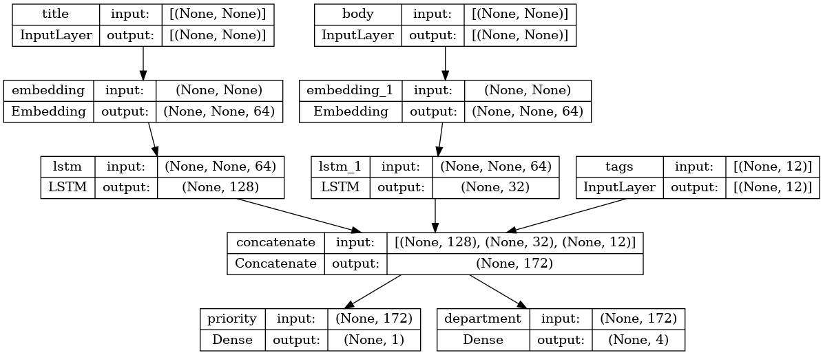
では、モデルをプロットします。
keras.utils.plot_model(model, "multi_input_and_output_model.png", show_shapes=True)
このモデルをコンパイルする時に、各出力に異なる損失を割り当てることができます。また、各損失に異なる重みを割り当てて、トレーニング損失全体へのそれらの寄与をモジュール化することも可能です。
model.compile(
    optimizer=keras.optimizers.RMSprop(1e-3),
    loss=[
        keras.losses.BinaryCrossentropy(from_logits=True),
        keras.losses.CategoricalCrossentropy(from_logits=True),
    ],
    loss_weights=[1.0, 0.2],
)
出力レイヤーの名前が異なるため、対応するレイヤー名を使用して、損失と損失の重みを指定することも可能です。
model.compile(
    optimizer=keras.optimizers.RMSprop(1e-3),
    loss={
        "priority": keras.losses.BinaryCrossentropy(from_logits=True),
        "department": keras.losses.CategoricalCrossentropy(from_logits=True),
    },
    loss_weights={"priority": 1.0, "department": 0.2},
)
入力とターゲットの NumPy 配列のリストを渡し、モデルをトレーニングします。
# Dummy input data
title_data = np.random.randint(num_words, size=(1280, 10))
body_data = np.random.randint(num_words, size=(1280, 100))
tags_data = np.random.randint(2, size=(1280, num_tags)).astype("float32")

# Dummy target data
priority_targets = np.random.random(size=(1280, 1))
dept_targets = np.random.randint(2, size=(1280, num_departments))

model.fit(
    {"title": title_data, "body": body_data, "tags": tags_data},
    {"priority": priority_targets, "department": dept_targets},
    epochs=2,
    batch_size=32,
)
Epoch 1/2
40/40 [==============================] - 7s 88ms/step - loss: 1.2841 - priority_loss: 0.7063 - department_loss: 2.8890
Epoch 2/2
40/40 [==============================] - 2s 39ms/step - loss: 1.3025 - priority_loss: 0.7044 - department_loss: 2.9903
<keras.src.callbacks.History at 0x7f1efcb6efd0>
Datasetオブジェクトで fit を呼び出す時、それは([title_data, body_data, tags_data], [priority_targets, dept_targets])などのリストのタプル、または({'title': title_data, 'body': body_data, 'tags': tags_data}、{'priority': priority_targets, 'department': dept_targets})などのディクショナリのタプルを yield する必要があります。
さらに詳しい説明については、トレーニングと評価ガイドをご覧ください。
トイ ResNet モデル
複数の入力と出力を持つモデルに加えて、Functional API では非線形接続トポロジー、つまりシーケンシャルに接続されていないレイヤーを持つモデルの操作を容易にします。これはSequential API では扱うことができません。
これの一般的なユースケースは、残差接続です。これを実証するために、CIFAR10 向けのトイ ResNet モデルを構築してみましょう。
inputs = keras.Input(shape=(32, 32, 3), name="img")
x = layers.Conv2D(32, 3, activation="relu")(inputs)
x = layers.Conv2D(64, 3, activation="relu")(x)
block_1_output = layers.MaxPooling2D(3)(x)

x = layers.Conv2D(64, 3, activation="relu", padding="same")(block_1_output)
x = layers.Conv2D(64, 3, activation="relu", padding="same")(x)
block_2_output = layers.add([x, block_1_output])

x = layers.Conv2D(64, 3, activation="relu", padding="same")(block_2_output)
x = layers.Conv2D(64, 3, activation="relu", padding="same")(x)
block_3_output = layers.add([x, block_2_output])

x = layers.Conv2D(64, 3, activation="relu")(block_3_output)
x = layers.GlobalAveragePooling2D()(x)
x = layers.Dense(256, activation="relu")(x)
x = layers.Dropout(0.5)(x)
outputs = layers.Dense(10)(x)

model = keras.Model(inputs, outputs, name="toy_resnet")
model.summary()
Model: "toy_resnet"
__________________________________________________________________________________________________
 Layer (type)                Output Shape                 Param #   Connected to
==================================================================================================
 img (InputLayer)            [(None, 32, 32, 3)]          0         []

 conv2d_8 (Conv2D)           (None, 30, 30, 32)           896       ['img[0][0]']

 conv2d_9 (Conv2D)           (None, 28, 28, 64)           18496     ['conv2d_8[0][0]']

 max_pooling2d_2 (MaxPoolin  (None, 9, 9, 64)             0         ['conv2d_9[0][0]']
 g2D)

 conv2d_10 (Conv2D)          (None, 9, 9, 64)             36928     ['max_pooling2d_2[0][0]']

 conv2d_11 (Conv2D)          (None, 9, 9, 64)             36928     ['conv2d_10[0][0]']

 add (Add)                   (None, 9, 9, 64)             0         ['conv2d_11[0][0]',
                                                                     'max_pooling2d_2[0][0]']

 conv2d_12 (Conv2D)          (None, 9, 9, 64)             36928     ['add[0][0]']

 conv2d_13 (Conv2D)          (None, 9, 9, 64)             36928     ['conv2d_12[0][0]']

 add_1 (Add)                 (None, 9, 9, 64)             0         ['conv2d_13[0][0]',
                                                                     'add[0][0]']

 conv2d_14 (Conv2D)          (None, 7, 7, 64)             36928     ['add_1[0][0]']

 global_average_pooling2d (  (None, 64)                   0         ['conv2d_14[0][0]']
 GlobalAveragePooling2D)

 dense_6 (Dense)             (None, 256)                  16640     ['global_average_pooling2d[0][
                                                                    0]']

 dropout (Dropout)           (None, 256)                  0         ['dense_6[0][0]']

 dense_7 (Dense)             (None, 10)                   2570      ['dropout[0][0]']

==================================================================================================
Total params: 223242 (872.04 KB)
Trainable params: 223242 (872.04 KB)
Non-trainable params: 0 (0.00 Byte)
__________________________________________________________________________________________________
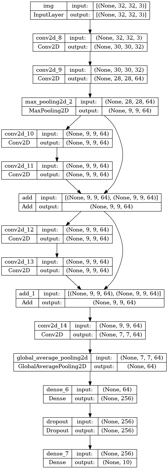
モデルをプロットします。
keras.utils.plot_model(model, "mini_resnet.png", show_shapes=True)
モデルをトレーニングします。
(x_train, y_train), (x_test, y_test) = keras.datasets.cifar10.load_data()

x_train = x_train.astype("float32") / 255.0
x_test = x_test.astype("float32") / 255.0
y_train = keras.utils.to_categorical(y_train, 10)
y_test = keras.utils.to_categorical(y_test, 10)

model.compile(
    optimizer=keras.optimizers.RMSprop(1e-3),
    loss=keras.losses.CategoricalCrossentropy(from_logits=True),
    metrics=["acc"],
)
# We restrict the data to the first 1000 samples so as to limit execution time
# on Colab. Try to train on the entire dataset until convergence!
model.fit(x_train[:1000], y_train[:1000], batch_size=64, epochs=1, validation_split=0.2)
Downloading data from https://www.cs.toronto.edu/~kriz/cifar-10-python.tar.gz
170498071/170498071 [==============================] - 2s 0us/step
13/13 [==============================] - 4s 80ms/step - loss: 2.3002 - acc: 0.1050 - val_loss: 2.2924 - val_acc: 0.1050
<keras.src.callbacks.History at 0x7f1efdc4a910>
レイヤーを共有する
Functional API のもう 1 つの良い使い方は、共有レイヤーを使用するモデルです。共有レイヤーは、同じモデルで複数回再利用されるレイヤーインスタンスのことで、レイヤーグラフ内の複数のパスに対応するフィーチャを学習します。
共有レイヤーは、似たような空間からの入力(例えば、似た語彙を特徴とする 2 つの異なるテキスト)をエンコードするためにしばしば使用されます。これにより、それら異なる入力間での情報の共有を可能になり、より少ないデータでそのようなモデルをトレーニングすることが可能になります。与えられた単語が入力のいずれかに見られる場合、それは共有レイヤーを通過する全ての入力の処理に有用です。
Functional API でレイヤーを共有するには、同じレイヤーインスタンスを複数回呼び出します。例えば、2 つの異なるテキスト入力間で共有される Embedding レイヤを以下に示します。
# Embedding for 1000 unique words mapped to 128-dimensional vectors
shared_embedding = layers.Embedding(1000, 128)

# Variable-length sequence of integers
text_input_a = keras.Input(shape=(None,), dtype="int32")

# Variable-length sequence of integers
text_input_b = keras.Input(shape=(None,), dtype="int32")

# Reuse the same layer to encode both inputs
encoded_input_a = shared_embedding(text_input_a)
encoded_input_b = shared_embedding(text_input_b)
レイヤーのグラフのノードを抽出して再利用する
操作しているレイヤーのグラフは静的なデータ構造であるため、アクセスして検査をすることができます。そして、これが関数型モデルを画像としてプロットする方法でもあります。
これはまた、中間レイヤー(グラフ内の「ノード」)のアクティブ化にアクセスが可能で、他の場所で再利用できることを意味します。これは特徴抽出などに非常に便利です。
例を見てみましょう。これは ImageNet 上で事前トレーニングされた、重みを持つ VGG19 モデルです。
vgg19 = tf.keras.applications.VGG19()
Downloading data from https://storage.googleapis.com/tensorflow/keras-applications/vgg19/vgg19_weights_tf_dim_ordering_tf_kernels.h5
574710816/574710816 [==============================] - 2s 0us/step
そしてこれらはグラフデータ構造をクエリして得られる、モデルの中間的なアクティブ化です。
features_list = [layer.output for layer in vgg19.layers]
これらの機能を使用して、中間レイヤーのアクティブ化の値を返す新しい特徴抽出モデルを作成します。
feat_extraction_model = keras.Model(inputs=vgg19.input, outputs=features_list)

img = np.random.random((1, 224, 224, 3)).astype("float32")
extracted_features = feat_extraction_model(img)
これは特に、ニューラルスタイル転送などのタスクに有用です。
カスタム層を使用して API を拡張する
tf.kerasには、例えば、次のような幅広い組み込みレイヤーが含まれています。
- 畳み込みレイヤー :
Conv1D、Conv2D、Conv3D、Conv2DTranspose - Pooling レイヤー :
MaxPooling1D、MaxPooling2D、MaxPooling3D、AveragePooling1D - RNN レイヤー :
GRU、LSTM、ConvLSTM2D BatchNormalization、Dropout、Embedding、など
必要なものが見つからない場合は、独自のレイヤーを作成して容易に API を拡張することができます。すべてのレイヤーはLayerクラスをサブクラス化して実装します。
callメソッドは、レイヤーが行う計算を指定します。buildメソッドは、レイヤーの重みを作成します(__init__でも重みを作成できるため、これは単なるスタイル慣習です)。
レイヤーの新規作成に関する詳細については、カスタムレイヤーとモデルガイドをご覧ください。
tf.keras.layers.Denseの基本的な実装を以下に示します。
class CustomDense(layers.Layer):
    def __init__(self, units=32):
        super(CustomDense, self).__init__()
        self.units = units

    def build(self, input_shape):
        self.w = self.add_weight(
            shape=(input_shape[-1], self.units),
            initializer="random_normal",
            trainable=True,
        )
        self.b = self.add_weight(
            shape=(self.units,), initializer="random_normal", trainable=True
        )

    def call(self, inputs):
        return tf.matmul(inputs, self.w) + self.b


inputs = keras.Input((4,))
outputs = CustomDense(10)(inputs)

model = keras.Model(inputs, outputs)
カスタムレイヤーでシリアル化をサポートするには、レイヤーインスタンスのコンストラクタ引数を返す get_config メソッドを定義します。
class CustomDense(layers.Layer):
    def __init__(self, units=32):
        super(CustomDense, self).__init__()
        self.units = units

    def build(self, input_shape):
        self.w = self.add_weight(
            shape=(input_shape[-1], self.units),
            initializer="random_normal",
            trainable=True,
        )
        self.b = self.add_weight(
            shape=(self.units,), initializer="random_normal", trainable=True
        )

    def call(self, inputs):
        return tf.matmul(inputs, self.w) + self.b

    def get_config(self):
        return {"units": self.units}


inputs = keras.Input((4,))
outputs = CustomDense(10)(inputs)

model = keras.Model(inputs, outputs)
config = model.get_config()

new_model = keras.Model.from_config(config, custom_objects={"CustomDense": CustomDense})
オプションで、config ディクショナリが与えられたレイヤーインスタンスを再作成する際に使用されたクラスメソッド from_config(cls, config) を実装します。デフォルトの from_config の実装は以下の通りです。
def from_config(cls, config):
  return cls(**config)
いつ Functional API を使用するか
新しいモデルを作成する場合または Modelクラスを直接サブクラス化する場合に、Keras Functional API を使用する必要があるのでしょうか? 一般的に Functional API はより高レベル、より容易かつ安全で、サブクラス化されたモデルがサポートしない多くの特徴を持っています。
ただし、レイヤーの有向非巡回グラフ(DAG)として容易に表現できないモデルを構築する場合には、モデルのサブクラス化がより大きな柔軟性を与えます。例えば、Functional API では Tree-RNN を実装できず、Modelを直接サブクラス化する必要があります。
Functional API とモデルのサブクラス化の違いに関する詳細については、TensorFlow 2.0 における Symbolic API と Imperative API とは?をご覧ください。
Functional API の長所 :
以下のプロパティは、(データ構造体でもある)Sequential モデルには真であり、(Python のバイトコードであり、データ構造体ではない)サブクラス化されたモデルには真ではありません。
低い冗長性
super(MyClass, self).__init__(...)、def call(self, ...):などがありません。
比較しよう :
inputs = keras.Input(shape=(32,))
x = layers.Dense(64, activation='relu')(inputs)
outputs = layers.Dense(10)(x)
mlp = keras.Model(inputs, outputs)
サブクラス化されたバージョンと比べます。
class MLP(keras.Model):

  def __init__(self, **kwargs):
    super(MLP, self).__init__(**kwargs)
    self.dense_1 = layers.Dense(64, activation='relu')
    self.dense_2 = layers.Dense(10)

  def call(self, inputs):
    x = self.dense_1(inputs)
    return self.dense_2(x)

# Instantiate the model.
mlp = MLP()
# Necessary to create the model's state.
# The model doesn't have a state until it's called at least once.
_ = mlp(tf.zeros((1, 32)))
連結グラフを定義しながらモデルを検証する
Functional API では、入力仕様(形状とdtype)が(Inputを使用して)あらかじめ作成されています。レイヤーを呼び出すたびに、レイヤーは渡された仕様が想定と一致しているかどうかをチェックし、一致していない場合には有用なエラーメッセージを表示します。
これにより、Functional API を使用して構築できるモデルは全て確実に実行されます。収束関連のデバッグ以外の全てのデバッグは、実行時ではなく、モデル構築中に静的に行われます。これはコンパイラの型チェックに類似しています。
関数型モデルはプロット可能かつ検査可能です
モデルをグラフとしてプロットすることが可能で、このグラフの中間ノードに簡単にアクセスすることができます。例えば(前の例で示したように)中間レイヤーのアクティブ化を抽出して再利用します。
features_list = [layer.output for layer in vgg19.layers]
feat_extraction_model = keras.Model(inputs=vgg19.input, outputs=features_list)
関数型モデルは、シリアル化やクローン化が可能です
関数型モデルはコードの一部ではなくデータ構造であるため、安全なシリアル化が可能です。また、単一のファイルとして保存できるため、元のコードにアクセスすることなく全く同じモデルを再作成することができます。詳細はシリアル化と保存に関するガイドをご覧ください。
サブクラス化されたモデルをシリアライズするには、実装者がモデルレベルでget_config()およびfrom_config()メソッドを指定する必要があります。
Functional API の弱点 :
動的アーキテクチャをサポートしません
Functional API は、モデルをレイヤーの DAG として扱います。これはほとんどのディープラーニングアーキテクチャでは真ですが、必ずしも全てのアーキテクチャに該当するわけではありません。例えば、再帰的ネットワークや Tree RNN はこの想定に従わないため、Functional API では実装できません。
異なる API スタイルをうまく組み合わせる
Functional API とモデルのサブクラス化のいずれかを選択することは、モデルの 1 つのカテゴリに制限する二者択一ではありません。tf.keras API 内の全てのモデルは、それらがSequential モデルでも、関数型モデルでも、新規に書かれたサブクラス化されたモデルであっても、お互いに相互作用することができます。
関数型モデルやSequentialモデルは、サブクラス化されたモデルやレイヤーの一部として常に使用することができます。
units = 32
timesteps = 10
input_dim = 5

# Define a Functional model
inputs = keras.Input((None, units))
x = layers.GlobalAveragePooling1D()(inputs)
outputs = layers.Dense(1)(x)
model = keras.Model(inputs, outputs)


class CustomRNN(layers.Layer):
    def __init__(self):
        super(CustomRNN, self).__init__()
        self.units = units
        self.projection_1 = layers.Dense(units=units, activation="tanh")
        self.projection_2 = layers.Dense(units=units, activation="tanh")
        # Our previously-defined Functional model
        self.classifier = model

    def call(self, inputs):
        outputs = []
        state = tf.zeros(shape=(inputs.shape[0], self.units))
        for t in range(inputs.shape[1]):
            x = inputs[:, t, :]
            h = self.projection_1(x)
            y = h + self.projection_2(state)
            state = y
            outputs.append(y)
        features = tf.stack(outputs, axis=1)
        print(features.shape)
        return self.classifier(features)


rnn_model = CustomRNN()
_ = rnn_model(tf.zeros((1, timesteps, input_dim)))
(1, 10, 32)
次のいずれかのパターンに従ったcallメソッドを実装していれば、Functional API で任意のサブクラス化されたレイヤーやモデルを使用することができます。
call(self, inputs, **kwargs)-- ここでいうinputsは、テンソルまたはテンソルのネストされた構造(テンソルのリストなど)であり、**kwargsは非テンソルの引数(非 inputs)です。call(self, inputs, training=None, **kwargs)-- このtrainingは、レイヤーがトレーニングモードと推論モードで振る舞うべきかどうかを示すブールです。call(self, inputs, mask=None, **kwargs)-- このmaskは、ブールマスクテンソルです。(例えば RNNに便利です。)call(self, inputs, training=None, mask=None, **kwargs)-- もちろん、マスキングとトレーニング固有の動作の両方を同時に持つことができます。
さらに、カスタムレイヤーやモデルでget_configメソッドを実装する場合、作成した関数型モデルは依然としてシリアル化やクローン化が可能です。
新規に書かれたカスタム RNN を関数型モデルで使用する簡単な例を以下に示します。
units = 32
timesteps = 10
input_dim = 5
batch_size = 16


class CustomRNN(layers.Layer):
    def __init__(self):
        super(CustomRNN, self).__init__()
        self.units = units
        self.projection_1 = layers.Dense(units=units, activation="tanh")
        self.projection_2 = layers.Dense(units=units, activation="tanh")
        self.classifier = layers.Dense(1)

    def call(self, inputs):
        outputs = []
        state = tf.zeros(shape=(inputs.shape[0], self.units))
        for t in range(inputs.shape[1]):
            x = inputs[:, t, :]
            h = self.projection_1(x)
            y = h + self.projection_2(state)
            state = y
            outputs.append(y)
        features = tf.stack(outputs, axis=1)
        return self.classifier(features)


# Note that you specify a static batch size for the inputs with the `batch_shape`
# arg, because the inner computation of `CustomRNN` requires a static batch size
# (when you create the `state` zeros tensor).
inputs = keras.Input(batch_shape=(batch_size, timesteps, input_dim))
x = layers.Conv1D(32, 3)(inputs)
outputs = CustomRNN()(x)

model = keras.Model(inputs, outputs)

rnn_model = CustomRNN()
_ = rnn_model(tf.zeros((1, 10, 5)))