
 GitHub에서 소스 보기 GitHub에서 소스 보기 |
설정
import tensorflow as tf
from tensorflow import keras
from tensorflow.keras import layers
2022-12-14 22:59:44.829135: W tensorflow/compiler/xla/stream_executor/platform/default/dso_loader.cc:64] Could not load dynamic library 'libnvinfer.so.7'; dlerror: libnvinfer.so.7: cannot open shared object file: No such file or directory
2022-12-14 22:59:44.829246: W tensorflow/compiler/xla/stream_executor/platform/default/dso_loader.cc:64] Could not load dynamic library 'libnvinfer_plugin.so.7'; dlerror: libnvinfer_plugin.so.7: cannot open shared object file: No such file or directory
2022-12-14 22:59:44.829257: W tensorflow/compiler/tf2tensorrt/utils/py_utils.cc:38] TF-TRT Warning: Cannot dlopen some TensorRT libraries. If you would like to use Nvidia GPU with TensorRT, please make sure the missing libraries mentioned above are installed properly.
시작하기
이 안내서는 훈련 및 유효성 검증을 위해 내장 API를 사용할 때의 훈련, 평가 및 예측(추론) 모델(예: model.fit(), model.evaluate(), model.predict())에 대해 설명합니다.
고유한 훈련 스텝 함수를 지정하면서 fit()을 사용하려면 fit()에서 이루어지는 작업 사용자 정의하기 가이드를 참조하세요.
고유한 훈련 및 평가 루프를 처음부터 작성하려면 "처음부터 훈련 루프 작성" 안내서를 참조하세요.
일반적으로, 내장 루프를 사용하든 직접 작성하든 관계없이 모델 훈련 및 유효성 검사는 모든 종류의 Keras 모델(순차 모델, Functional API로 작성된 모델 및 모델 하위 클래스화를 통해 처음부터 작성된 모델)에서 완전히 동일하게 작동합니다.
이 안내서는 분산 훈련에 대해서는 다루지 않습니다. 이 부분은 멀티 GPU 및 분산 교육 안내서를 참조하세요.
API 개요: 첫 번째 엔드 투 엔드 예제
데이터를 모델의 내장 훈련 루프로 전달할 때는 NumPy 배열(데이터가 작고 메모리에 맞는 경우) 또는 tf.data Dataset 객체를 사용해야 합니다. 다음 몇 단락에서는 옵티마이저, 손실 및 메트릭을 사용하는 방법을 보여주기 위해 MNIST 데이터세트를 NumPy 배열로 사용하겠습니다.
다음 모델을 고려해 보겠습니다(여기서는 Functional API를 사용하여 빌드하지만 시퀀스 모델 또는 하위 클래스화된 모델도 가능함).
inputs = keras.Input(shape=(784,), name="digits")
x = layers.Dense(64, activation="relu", name="dense_1")(inputs)
x = layers.Dense(64, activation="relu", name="dense_2")(x)
outputs = layers.Dense(10, activation="softmax", name="predictions")(x)

model = keras.Model(inputs=inputs, outputs=outputs)
일반적인 엔드 투 엔드 워크플로는 다음과 같이 구성됩니다.
- 훈련
- 원래 훈련 데이터에서 생성된 홀드아웃 세트에 대한 유효성 검사
- 테스트 데이터에 대한 평가
이 예에서는 MNIST 데이터를 사용합니다.
(x_train, y_train), (x_test, y_test) = keras.datasets.mnist.load_data()

# Preprocess the data (these are NumPy arrays)
x_train = x_train.reshape(60000, 784).astype("float32") / 255
x_test = x_test.reshape(10000, 784).astype("float32") / 255

y_train = y_train.astype("float32")
y_test = y_test.astype("float32")

# Reserve 10,000 samples for validation
x_val = x_train[-10000:]
y_val = y_train[-10000:]
x_train = x_train[:-10000]
y_train = y_train[:-10000]
훈련 구성(최적화 프로그램, 손실, 메트릭)을 지정합니다.
model.compile(
    optimizer=keras.optimizers.RMSprop(),  # Optimizer
    # Loss function to minimize
    loss=keras.losses.SparseCategoricalCrossentropy(),
    # List of metrics to monitor
    metrics=[keras.metrics.SparseCategoricalAccuracy()],
)
fit()를 호출하여 데이터를 batch_size 크기의 "배치"로 분할하고 지정된 수의 epochs에 대해 전체 데이터세트를 반복 처리하여 모델을 훈련시킵니다.
print("Fit model on training data")
history = model.fit(
    x_train,
    y_train,
    batch_size=64,
    epochs=2,
    # We pass some validation for
    # monitoring validation loss and metrics
    # at the end of each epoch
    validation_data=(x_val, y_val),
)
Fit model on training data
Epoch 1/2
782/782 [==============================] - 3s 3ms/step - loss: 0.3338 - sparse_categorical_accuracy: 0.9047 - val_loss: 0.1792 - val_sparse_categorical_accuracy: 0.9496
Epoch 2/2
782/782 [==============================] - 2s 3ms/step - loss: 0.1635 - sparse_categorical_accuracy: 0.9516 - val_loss: 0.1278 - val_sparse_categorical_accuracy: 0.9632
반환되는 history 객체는 훈련 중 손실 값과 메트릭 값에 대한 레코드를 유지합니다.
history.history
{'loss': [0.3337874710559845, 0.16347293555736542],
 'sparse_categorical_accuracy': [0.9046599864959717, 0.9516400098800659],
 'val_loss': [0.17921485006809235, 0.12782561779022217],
 'val_sparse_categorical_accuracy': [0.9495999813079834, 0.9631999731063843]}
evaluate()를 통해 테스트 데이터에 대해 모델을 평가합니다.
# Evaluate the model on the test data using `evaluate`
print("Evaluate on test data")
results = model.evaluate(x_test, y_test, batch_size=128)
print("test loss, test acc:", results)

# Generate predictions (probabilities -- the output of the last layer)
# on new data using `predict`
print("Generate predictions for 3 samples")
predictions = model.predict(x_test[:3])
print("predictions shape:", predictions.shape)
79/79 [==============================] - 0s 2ms/step - loss: 0.1320 - sparse_categorical_accuracy: 0.9597
1/1 [==============================] - 0s 71ms/step
predictions shape: (3, 10)
이제 이 워크플로의 각 부분을 자세히 살펴보겠습니다.
compile() 메서드: 손실, 메트릭 및 최적화 프로그램 지정하기
fit()으로 모델을 훈련시키려면 손실 함수, 최적화 프로그램, 그리고 선택적으로 모니터링할 일부 메트릭을 지정해야 합니다.
이러한 내용은 compile() 메서드에 대한 인수로 모델에 전달합니다.
model.compile(
    optimizer=keras.optimizers.RMSprop(learning_rate=1e-3),
    loss=keras.losses.SparseCategoricalCrossentropy(),
    metrics=[keras.metrics.SparseCategoricalAccuracy()],
)
metrics 인수는 목록이어야 합니다. 모델의 메트릭 수는 얼마든지 가능합니다.
모델에 여러 개의 출력이 있는 경우 각 출력에 대해 서로 다른 손실 및 메트릭을 지정하고 모델의 총 손실에 대한 각 출력의 기여도를 조정할 수 있습니다. 이에 대한 자세한 내용은 다중 입력, 다중 출력 모델로 데이터 전달 섹션에서 확인할 수 있습니다.
기본 설정에 문제가 없으면 대부분의 경우 최적화 프로그램, 손실 및 메트릭을 문자열 식별자를 통해 바로 가기로 지정할 수 있습니다.
model.compile(
    optimizer="rmsprop",
    loss="sparse_categorical_crossentropy",
    metrics=["sparse_categorical_accuracy"],
)
나중에 재사용하기 위해 모델 정의와 컴파일 단계를 함수에 넣겠습니다. 이 안내서의 여러 예에서 여러 번 호출합니다.
def get_uncompiled_model():
    inputs = keras.Input(shape=(784,), name="digits")
    x = layers.Dense(64, activation="relu", name="dense_1")(inputs)
    x = layers.Dense(64, activation="relu", name="dense_2")(x)
    outputs = layers.Dense(10, activation="softmax", name="predictions")(x)
    model = keras.Model(inputs=inputs, outputs=outputs)
    return model


def get_compiled_model():
    model = get_uncompiled_model()
    model.compile(
        optimizer="rmsprop",
        loss="sparse_categorical_crossentropy",
        metrics=["sparse_categorical_accuracy"],
    )
    return model
많은 내장 최적화 프로그램, 손실 및 메트릭을 사용할 수 있습니다
일반적으로 고유한 손실, 메트릭 또는 최적화 프로그램을 처음부터 새로 만들 필요가 없는데, Keras API에 필요한 것들이 이미 들어 있을 개연성이 높기 때문입니다.
최적화 프로그램:
SGD()(모멘텀이 있거나 없음)RMSprop()Adam()- 기타
손실:
MeanSquaredError()KLDivergence()CosineSimilarity()- 기타
메트릭:
AUC()Precision()Recall()- 기타
사용자 정의 손실
사용자 정의 손실을 만들어야 하는 경우 Keras는 이를 수행하는 두 가지 방법을 제공합니다.
첫 번째 예는 입력 y_true 및 y_pred를 받아들이는 함수를 만듭니다. 다음 예는 실제 데이터와 예측 사이의 오차에 대한 평균 제곱을 계산하는 손실 함수를 보여줍니다.
def custom_mean_squared_error(y_true, y_pred):
    return tf.math.reduce_mean(tf.square(y_true - y_pred))


model = get_uncompiled_model()
model.compile(optimizer=keras.optimizers.Adam(), loss=custom_mean_squared_error)

# We need to one-hot encode the labels to use MSE
y_train_one_hot = tf.one_hot(y_train, depth=10)
model.fit(x_train, y_train_one_hot, batch_size=64, epochs=1)
782/782 [==============================] - 3s 2ms/step - loss: 0.0164
<keras.callbacks.History at 0x7ff4700906d0>
y_true 및 y_pred 이외의 매개변수를 사용하는 손실 함수가 필요한 경우 tf.keras.losses.Loss 클래스를 하위 클래스화하고 다음 두 메서드를 구현할 수 있습니다.
__init__(self): 손실 함수 호출 중에 전달할 매개변수를 받아들입니다.call(self, y_true, y_pred): 목표(y_true)와 모델 예측(y_pred)을 사용하여 모델의 손실을 계산합니다.
오차의 평균 제곱을 사용하려고 하지만 예측 값을 0.5에서 멀어지게 하는 항이 추가되었다고 가정해 보겠습니다(범주형 목표가 원-핫 인코딩되고 0과 1 사이의 값을 취하는 것으로 가정). 이렇게 하면 모델이 너무 확신을 갖지 않게 하는 인센티브가 생겨 과적합을 줄이는 데 도움이 될 수 있습니다(시도해 보기 전에는 효과가 있는지 알 수 없음).
방법은 다음과 같습니다.
class CustomMSE(keras.losses.Loss):
    def __init__(self, regularization_factor=0.1, name="custom_mse"):
        super().__init__(name=name)
        self.regularization_factor = regularization_factor

    def call(self, y_true, y_pred):
        mse = tf.math.reduce_mean(tf.square(y_true - y_pred))
        reg = tf.math.reduce_mean(tf.square(0.5 - y_pred))
        return mse + reg * self.regularization_factor


model = get_uncompiled_model()
model.compile(optimizer=keras.optimizers.Adam(), loss=CustomMSE())

y_train_one_hot = tf.one_hot(y_train, depth=10)
model.fit(x_train, y_train_one_hot, batch_size=64, epochs=1)
782/782 [==============================] - 3s 2ms/step - loss: 0.0384
<keras.callbacks.History at 0x7ff3fc3e46d0>
사용자 정의 메트릭
API의 일부가 아닌 메트릭이 필요한 경우 tf.keras.metrics.Metric 클래스를 하위 클래스화하여 사용자 정의 메트릭을 쉽게 생성할 수 있습니다. 다음과 같은 4가지 메서드를 구현해야 합니다.
__init__(self). 메트릭에 대한 상태 변수를 생성합니다.update_state(self, y_true, y_pred, sample_weight=None). y_true 목표값과 y_pred 모델 예측값을 사용하여 상태 변수를 업데이트합니다.result(self). 상태 변수를 사용하여 최종 경과를 계산합니다.reset_state(self). 메트릭 상태를 다시 초기화합니다.
상태 업데이트와 결과 계산은 개별적으로 수행됩니다(각각 update_state() 및 result() 사용). 이는 일부의 경우 결과 계산 부담이 매우 크며 주기적으로만 수행되기 때문입니다.
다음은 제공된 클래스에 속해있는 것으로 올바르게 분류된 샘플 수를 계산하는 CategoricalTruePositives 메트릭을 구현하는 방법을 보여주는 간단한 예시입니다.
class CategoricalTruePositives(keras.metrics.Metric):
    def __init__(self, name="categorical_true_positives", **kwargs):
        super(CategoricalTruePositives, self).__init__(name=name, **kwargs)
        self.true_positives = self.add_weight(name="ctp", initializer="zeros")

    def update_state(self, y_true, y_pred, sample_weight=None):
        y_pred = tf.reshape(tf.argmax(y_pred, axis=1), shape=(-1, 1))
        values = tf.cast(y_true, "int32") == tf.cast(y_pred, "int32")
        values = tf.cast(values, "float32")
        if sample_weight is not None:
            sample_weight = tf.cast(sample_weight, "float32")
            values = tf.multiply(values, sample_weight)
        self.true_positives.assign_add(tf.reduce_sum(values))

    def result(self):
        return self.true_positives

    def reset_state(self):
        # The state of the metric will be reset at the start of each epoch.
        self.true_positives.assign(0.0)


model = get_uncompiled_model()
model.compile(
    optimizer=keras.optimizers.RMSprop(learning_rate=1e-3),
    loss=keras.losses.SparseCategoricalCrossentropy(),
    metrics=[CategoricalTruePositives()],
)
model.fit(x_train, y_train, batch_size=64, epochs=3)
Epoch 1/3
782/782 [==============================] - 2s 2ms/step - loss: 0.3449 - categorical_true_positives: 45113.0000
Epoch 2/3
782/782 [==============================] - 2s 2ms/step - loss: 0.1612 - categorical_true_positives: 47543.0000
Epoch 3/3
782/782 [==============================] - 2s 2ms/step - loss: 0.1155 - categorical_true_positives: 48232.0000
<keras.callbacks.History at 0x7ff3fc301100>
표준 서명에 맞지 않는 손실 및 메트릭 처리하기
거의 대부분의 손실과 메트릭은 y_true 및 y_pred에서 계산할 수 있습니다(여기서 y_pred가 모델의 출력). 그러나 모두가 그런 것은 아닙니다. 예를 들어, 정규화 손실은 레이어의 활성화만 요구할 수 있으며(이 경우 목표가 없음) 이 활성화는 모델 출력이 아닐 수 있습니다.
이러한 경우 사용자 정의 레이어의 호출 메서드 내에서 self.add_loss(loss_value)를 호출할 수 있습니다. 이러한 방식으로 추가된 손실은 훈련 중 "주요" 손실(compile()로 전달되는 손실)에 추가됩니다. 다음은 활동 정규화를 추가하는 간단한 예입니다. 참고로 활동 정규화는 모든 Keras 레이어에 내장되어 있으며 이 레이어는 구체적인 예를 제공하기 위한 것입니다.
class ActivityRegularizationLayer(layers.Layer):
    def call(self, inputs):
        self.add_loss(tf.reduce_sum(inputs) * 0.1)
        return inputs  # Pass-through layer.


inputs = keras.Input(shape=(784,), name="digits")
x = layers.Dense(64, activation="relu", name="dense_1")(inputs)

# Insert activity regularization as a layer
x = ActivityRegularizationLayer()(x)

x = layers.Dense(64, activation="relu", name="dense_2")(x)
outputs = layers.Dense(10, name="predictions")(x)

model = keras.Model(inputs=inputs, outputs=outputs)
model.compile(
    optimizer=keras.optimizers.RMSprop(learning_rate=1e-3),
    loss=keras.losses.SparseCategoricalCrossentropy(from_logits=True),
)

# The displayed loss will be much higher than before
# due to the regularization component.
model.fit(x_train, y_train, batch_size=64, epochs=1)
782/782 [==============================] - 2s 2ms/step - loss: 2.5129
<keras.callbacks.History at 0x7ff3fc17eb80>
add_metric()을 사용하여 메트릭 값 로깅에 대해 같은 작업을 수행할 수 있습니다.
class MetricLoggingLayer(layers.Layer):
    def call(self, inputs):
        # The `aggregation` argument defines
        # how to aggregate the per-batch values
        # over each epoch:
        # in this case we simply average them.
        self.add_metric(
            keras.backend.std(inputs), name="std_of_activation", aggregation="mean"
        )
        return inputs  # Pass-through layer.


inputs = keras.Input(shape=(784,), name="digits")
x = layers.Dense(64, activation="relu", name="dense_1")(inputs)

# Insert std logging as a layer.
x = MetricLoggingLayer()(x)

x = layers.Dense(64, activation="relu", name="dense_2")(x)
outputs = layers.Dense(10, name="predictions")(x)

model = keras.Model(inputs=inputs, outputs=outputs)
model.compile(
    optimizer=keras.optimizers.RMSprop(learning_rate=1e-3),
    loss=keras.losses.SparseCategoricalCrossentropy(from_logits=True),
)
model.fit(x_train, y_train, batch_size=64, epochs=1)
782/782 [==============================] - 2s 2ms/step - loss: 0.3300 - std_of_activation: 0.9821
<keras.callbacks.History at 0x7ff3e433b1c0>
Functional API에서 model.add_loss(loss_tensor) 또는 model.add_metric(metric_tensor, name, aggregation)을 호출할 수도 있습니다.
다음은 간단한 예입니다.
inputs = keras.Input(shape=(784,), name="digits")
x1 = layers.Dense(64, activation="relu", name="dense_1")(inputs)
x2 = layers.Dense(64, activation="relu", name="dense_2")(x1)
outputs = layers.Dense(10, name="predictions")(x2)
model = keras.Model(inputs=inputs, outputs=outputs)

model.add_loss(tf.reduce_sum(x1) * 0.1)

model.add_metric(keras.backend.std(x1), name="std_of_activation", aggregation="mean")

model.compile(
    optimizer=keras.optimizers.RMSprop(1e-3),
    loss=keras.losses.SparseCategoricalCrossentropy(from_logits=True),
)
model.fit(x_train, y_train, batch_size=64, epochs=1)
782/782 [==============================] - 3s 2ms/step - loss: 2.5264 - std_of_activation: 0.0021
<keras.callbacks.History at 0x7ff3e41a1880>
add_loss()를 통해 손실을 전달하면 모델에 이미 최소화할 수 있는 손실이 있으므로 손실 함수 없이 compile()을 호출할 수 있습니다.
다음 LogisticEndpoint 레이어를 생각해 보겠습니다. 이 레이어는 입력으로 targets 및 logits를 받아들이고 add_loss()를 통해 교차 엔트로피 손실을 추적합니다. 또한 add_metric()를 통해 분류 정확도도 추적합니다.
class LogisticEndpoint(keras.layers.Layer):
    def __init__(self, name=None):
        super(LogisticEndpoint, self).__init__(name=name)
        self.loss_fn = keras.losses.BinaryCrossentropy(from_logits=True)
        self.accuracy_fn = keras.metrics.BinaryAccuracy()

    def call(self, targets, logits, sample_weights=None):
        # Compute the training-time loss value and add it
        # to the layer using `self.add_loss()`.
        loss = self.loss_fn(targets, logits, sample_weights)
        self.add_loss(loss)

        # Log accuracy as a metric and add it
        # to the layer using `self.add_metric()`.
        acc = self.accuracy_fn(targets, logits, sample_weights)
        self.add_metric(acc, name="accuracy")

        # Return the inference-time prediction tensor (for `.predict()`).
        return tf.nn.softmax(logits)
다음과 같이 loss 인수 없이 컴파일된 두 개의 입력(입력 data 및 targets)이 있는 모델에서 이를 사용할 수 있습니다.
import numpy as np

inputs = keras.Input(shape=(3,), name="inputs")
targets = keras.Input(shape=(10,), name="targets")
logits = keras.layers.Dense(10)(inputs)
predictions = LogisticEndpoint(name="predictions")(logits, targets)

model = keras.Model(inputs=[inputs, targets], outputs=predictions)
model.compile(optimizer="adam")  # No loss argument!

data = {
    "inputs": np.random.random((3, 3)),
    "targets": np.random.random((3, 10)),
}
model.fit(data)
1/1 [==============================] - 1s 511ms/step - loss: 1.0517 - binary_accuracy: 0.0000e+00
<keras.callbacks.History at 0x7ff3e4017d60>
다중 입력 모델의 훈련에 대한 자세한 내용은 다중 입력, 다중 출력 모델로 데이터 전달하기 섹션을 참조하세요.
유효성 검사 홀드아웃 세트를 자동으로 분리하기
앞서 보았던 첫 번째 엔드 투 엔드 예에서는 validation_data 인수를 사용하여 NumPy 배열의 튜플 (x_val, y_val)을 모델에 전달하여 각 epoch 끝에서 유효성 검사 손실과 유효성 검사 메트릭을 평가했습니다.
또 다른 옵션: 인수 validation_split를 사용하여 검증 목적으로 훈련 데이터의 일부를 자동으로 예약할 수 있습니다. 인수 값은 검증을 위해 예약할 데이터 비율을 나타내므로 0보다 크고 1보다 작은 값으로 설정해야 합니다. 예를 들어, validation_split=0.2는 "유효성 검사를 위해 데이터의 20%를 사용"한다는 의미이고validation_split=0.6은 "유효성 검사를 위해 데이터의 60%를 사용"한다는 의미입니다.
유효성을 계산하는 방법은 셔플링 전에 fit() 호출로 수신한 배열의 마지막 x% 샘플을 가져오는 것입니다.
NumPy 데이터로 훈련할 때만 validation_split을 사용할 수 있다는 점에 유의하세요.
model = get_compiled_model()
model.fit(x_train, y_train, batch_size=64, validation_split=0.2, epochs=1)
625/625 [==============================] - 2s 3ms/step - loss: 0.3722 - sparse_categorical_accuracy: 0.8945 - val_loss: 0.2303 - val_sparse_categorical_accuracy: 0.9323
<keras.callbacks.History at 0x7ff470137c70>
tf.data 데이터세트로부터 훈련 및 평가
앞서 몇 단락에 걸쳐 손실, 메트릭 및 옵티마이저를 처리하는 방법을 살펴보았으며, 데이터가 NumPy 배열로 전달될 때 fit()에서 validation_data 및 validation_split 인수를 사용하는 방법도 알아보았습니다.
이제 데이터가 tf.data.Dataset 객체의 형태로 제공되는 경우를 살펴보겠습니다.
tf.data API는 빠르고 확장 가능한 방식으로 데이터를 로드하고 사전 처리하기 위한 TensorFlow 2.0의 유틸리티 세트입니다.
Datasets 생성에 대한 자세한 설명은 tf.data 설명서를 참조하세요.
Dataset 인스턴스를 메서드 fit(), evaluate() 및 predict()로 직접 전달할 수 있습니다.
model = get_compiled_model()

# First, let's create a training Dataset instance.
# For the sake of our example, we'll use the same MNIST data as before.
train_dataset = tf.data.Dataset.from_tensor_slices((x_train, y_train))
# Shuffle and slice the dataset.
train_dataset = train_dataset.shuffle(buffer_size=1024).batch(64)

# Now we get a test dataset.
test_dataset = tf.data.Dataset.from_tensor_slices((x_test, y_test))
test_dataset = test_dataset.batch(64)

# Since the dataset already takes care of batching,
# we don't pass a `batch_size` argument.
model.fit(train_dataset, epochs=3)

# You can also evaluate or predict on a dataset.
print("Evaluate")
result = model.evaluate(test_dataset)
dict(zip(model.metrics_names, result))
Epoch 1/3
782/782 [==============================] - 2s 2ms/step - loss: 0.3543 - sparse_categorical_accuracy: 0.8999
Epoch 2/3
782/782 [==============================] - 2s 2ms/step - loss: 0.1725 - sparse_categorical_accuracy: 0.9486
Epoch 3/3
782/782 [==============================] - 2s 2ms/step - loss: 0.1259 - sparse_categorical_accuracy: 0.9618
Evaluate
157/157 [==============================] - 0s 2ms/step - loss: 0.1384 - sparse_categorical_accuracy: 0.9604
{'loss': 0.13835842907428741,
 'sparse_categorical_accuracy': 0.9603999853134155}
데이터세트는 각 epoch의 끝에서 재설정되므로 다음 epoch에서 재사용할 수 있습니다.
이 데이터세트의 특정 배치 수에 대해서만 훈련을 실행하려면 다음 epoch로 이동하기 전에 이 데이터세트를 사용하여 모델이 실행해야 하는 훈련 단계의 수를 지정하는 steps_per_epoch 인수를 전달할 수 있습니다.
이렇게 하면 각 epoch가 끝날 때 데이터세트가 재설정되지 않고 다음 배치를 계속 가져오게 됩니다. 무한 반복되는 데이터세트가 아니라면 결국 데이터세트의 데이터가 고갈됩니다.
model = get_compiled_model()

# Prepare the training dataset
train_dataset = tf.data.Dataset.from_tensor_slices((x_train, y_train))
train_dataset = train_dataset.shuffle(buffer_size=1024).batch(64)

# Only use the 100 batches per epoch (that's 64 * 100 samples)
model.fit(train_dataset, epochs=3, steps_per_epoch=100)
Epoch 1/3
100/100 [==============================] - 1s 2ms/step - loss: 0.8102 - sparse_categorical_accuracy: 0.7884
Epoch 2/3
100/100 [==============================] - 0s 2ms/step - loss: 0.3813 - sparse_categorical_accuracy: 0.8923
Epoch 3/3
100/100 [==============================] - 0s 2ms/step - loss: 0.3338 - sparse_categorical_accuracy: 0.9034
<keras.callbacks.History at 0x7ff3ac75cdf0>
유효성 검사 데이터세트 사용하기
fit()에서 Dataset 인스턴스를 validation_data 인수로 전달할 수 있습니다.
model = get_compiled_model()

# Prepare the training dataset
train_dataset = tf.data.Dataset.from_tensor_slices((x_train, y_train))
train_dataset = train_dataset.shuffle(buffer_size=1024).batch(64)

# Prepare the validation dataset
val_dataset = tf.data.Dataset.from_tensor_slices((x_val, y_val))
val_dataset = val_dataset.batch(64)

model.fit(train_dataset, epochs=1, validation_data=val_dataset)
782/782 [==============================] - 3s 3ms/step - loss: 0.3518 - sparse_categorical_accuracy: 0.9000 - val_loss: 0.1890 - val_sparse_categorical_accuracy: 0.9453
<keras.callbacks.History at 0x7ff3ac5789d0>
각 epoch가 끝날 때 모델은 검증 데이터세트를 반복하고 유효성 검사 손실 및 검증 메트릭을 계산합니다.
이 데이터세트의 특정 배치 수에 대해서만 유효성 검사를 실행하려면 유효성 검사를 중단하고 다음 epoch로 넘어가기 전에 유효성 검사 데이터세트에서 모델이 실행해야 하는 유효성 검사 단계의 수를 지정하는 validation_steps 인수를 전달할 수 있습니다.
model = get_compiled_model()

# Prepare the training dataset
train_dataset = tf.data.Dataset.from_tensor_slices((x_train, y_train))
train_dataset = train_dataset.shuffle(buffer_size=1024).batch(64)

# Prepare the validation dataset
val_dataset = tf.data.Dataset.from_tensor_slices((x_val, y_val))
val_dataset = val_dataset.batch(64)

model.fit(
    train_dataset,
    epochs=1,
    # Only run validation using the first 10 batches of the dataset
    # using the `validation_steps` argument
    validation_data=val_dataset,
    validation_steps=10,
)
782/782 [==============================] - 3s 2ms/step - loss: 0.3395 - sparse_categorical_accuracy: 0.9040 - val_loss: 0.2919 - val_sparse_categorical_accuracy: 0.9109
<keras.callbacks.History at 0x7ff3ac600340>
유효성 검사 데이터세트는 사용 후 매번 재설정되므로 epoch마다 항상 동일한 샘플을 평가하게 됩니다.
인수 validation_split(훈련 데이터로부터 홀드아웃 세트 생성)는 Dataset 객체로 훈련할 때는 지원되지 않는데, 이를 위해서는 데이터세트 샘플을 인덱싱할 수 있어야 하지만 Dataset API에서는 일반적으로 이것이 불가능하기 때문입니다.
지원되는 다른 입력 형식
NumPy 배열, 즉시 실행 텐서 및 TensorFlow Datasets 외에도 Pandas 데이터프레임을 사용하거나 데이터 및 레이블의 배치를 생성하는 Python 생성기에서 Keras 모델을 훈련할 수 있습니다.
특히, keras.utils.Sequence 클래스는 멀티스레딩을 인식하고 셔플이 가능한 Python 데이터 생성기를 빌드하기 위한 간단한 인터페이스를 제공합니다.
일반적으로 다음을 사용하는 것이 좋습니다.
- 데이터가 작고 메모리에 맞는 경우 NumPy 입력 데이터
- 큰 데이터세트가 있고 분산 훈련을 수행해야 하는 경우
Dataset객체 - 큰 데이터세트가 있고 TensorFlow에서 수행할 수 없는 많은 사용자 정의 Python 측 처리를 수행해야 하는 경우(예: 데이터 로드 또는 사전 처리를 위해 외부 라이브러리에 의존하는 경우)
Sequence객체
keras.utils.Sequence 객체를 입력으로 사용하기
keras.utils.Sequence는 두 가지 중요한 속성을 가진 Python 생성기를 얻기 위해 하위 클래스화를 수행할 수 있는 유틸리티입니다.
- 멀티 프로세싱과 잘 작동합니다.
- 셔플할 수 있습니다(예:
fit()에서shuffle=True를 전달하는 경우).
Sequence는 두 가지 메서드를 구현해야 합니다.
__getitem____len__
__getitem__ 메서드는 완전한 배치를 반환해야 합니다. epoch 사이에서 데이터세트를 수정하려면 on_epoch_end를 구현할 수 있습니다.
다음은 간단한 예입니다.
from skimage.io import imread
from skimage.transform import resize
import numpy as np

# Here, `filenames` is list of path to the images
# and `labels` are the associated labels.

class CIFAR10Sequence(Sequence):
    def __init__(self, filenames, labels, batch_size):
        self.filenames, self.labels = filenames, labels
        self.batch_size = batch_size

    def __len__(self):
        return int(np.ceil(len(self.filenames) / float(self.batch_size)))

    def __getitem__(self, idx):
        batch_x = self.filenames[idx * self.batch_size:(idx + 1) * self.batch_size]
        batch_y = self.labels[idx * self.batch_size:(idx + 1) * self.batch_size]
        return np.array([
            resize(imread(filename), (200, 200))
               for filename in batch_x]), np.array(batch_y)

sequence = CIFAR10Sequence(filenames, labels, batch_size)
model.fit(sequence, epochs=10)
샘플 가중치 및 클래스 가중치 사용하기
기본 설정에서는 샘플의 가중치가 데이터세트의 빈도에 따라 결정됩니다. 샘플 빈도와 관계없이 데이터에 가중치를 부여하는 방법에는 두 가지가 있습니다.
- 클래스 가중치
- 샘플 가중치
클래스 가중치
이 가중치는 Model.fit()에 대한 class_weight 인수로 사전을 전달하여 설정합니다. 이 사전은 클래스 인덱스를 이 클래스에 속한 샘플에 사용해야 하는 가중치에 매핑합니다.
이 방법은 샘플링을 다시 수행하지 않고 클래스의 균형을 맞추거나 특정 클래스에 더 중요한 모델을 훈련시키는 데 사용할 수 있습니다.
예를 들어, 데이터에서 클래스 "0"이 클래스 "1"로 표시된 것의 절반인 경우 Model.fit(..., class_weight={0: 1., 1: 0.5})을 사용할 수 있습니다.
다음은 클래스 #5(MNIST 데이터세트에서 숫자 "5")의 올바른 분류에 더 많은 중요성을 두도록 클래스 가중치 또는 샘플 가중치를 사용하는 NumPy 예입니다.
import numpy as np

class_weight = {
    0: 1.0,
    1: 1.0,
    2: 1.0,
    3: 1.0,
    4: 1.0,
    # Set weight "2" for class "5",
    # making this class 2x more important
    5: 2.0,
    6: 1.0,
    7: 1.0,
    8: 1.0,
    9: 1.0,
}

print("Fit with class weight")
model = get_compiled_model()
model.fit(x_train, y_train, class_weight=class_weight, batch_size=64, epochs=1)
Fit with class weight
782/782 [==============================] - 3s 2ms/step - loss: 0.3768 - sparse_categorical_accuracy: 0.9018
<keras.callbacks.History at 0x7ff3ac2eca30>
샘플 가중치
세밀한 제어가 필요하거나 분류기를 빌드하지 않는 경우 "샘플 가중치"를 사용할 수 있습니다.
- NumPy 데이터에서 훈련하는 경우:
sample_weight인수를Model.fit()으로 전달합니다. tf.data또는 다른 종류의 반복기에서 훈련하는 경우: Yield(input_batch, label_batch, sample_weight_batch)튜플을 생성합니다.
"샘플 가중치" 배열은 총 손실을 계산할 때 배치의 각 샘플에 필요한 가중치를 지정하는 숫자 배열로, 불균형적인 분류 문제에 일반적으로 사용됩니다(거의 드러나지 않는 클래스에 더 많은 가중치를 부여한다는 개념).
사용된 가중치가 1과 0인 경우, 배열은 손실 함수에 대한 마스크로 사용될 수 있습니다(전체 손실에 대한 특정 샘플의 기여도를 완전히 버림).
sample_weight = np.ones(shape=(len(y_train),))
sample_weight[y_train == 5] = 2.0

print("Fit with sample weight")
model = get_compiled_model()
model.fit(x_train, y_train, sample_weight=sample_weight, batch_size=64, epochs=1)
Fit with sample weight
782/782 [==============================] - 2s 2ms/step - loss: 0.3830 - sparse_categorical_accuracy: 0.8991
<keras.callbacks.History at 0x7ff3ac189b50>
다음은 이에 해당하는 Dataset의 예입니다.
sample_weight = np.ones(shape=(len(y_train),))
sample_weight[y_train == 5] = 2.0

# Create a Dataset that includes sample weights
# (3rd element in the return tuple).
train_dataset = tf.data.Dataset.from_tensor_slices((x_train, y_train, sample_weight))

# Shuffle and slice the dataset.
train_dataset = train_dataset.shuffle(buffer_size=1024).batch(64)

model = get_compiled_model()
model.fit(train_dataset, epochs=1)
782/782 [==============================] - 2s 2ms/step - loss: 0.3715 - sparse_categorical_accuracy: 0.9016
<keras.callbacks.History at 0x7ff3ac0a27f0>
다중 입력, 다중 출력 모델로 데이터 전달하기
이전 예에서는 단일 입력(형상 (764,)의 텐서)과 단일 출력(형상 (10,)의 예측 텐서)이 있는 모델을 고려했습니다. 그러나 입력 또는 출력이 여러 개인 모델은 어떨까요?
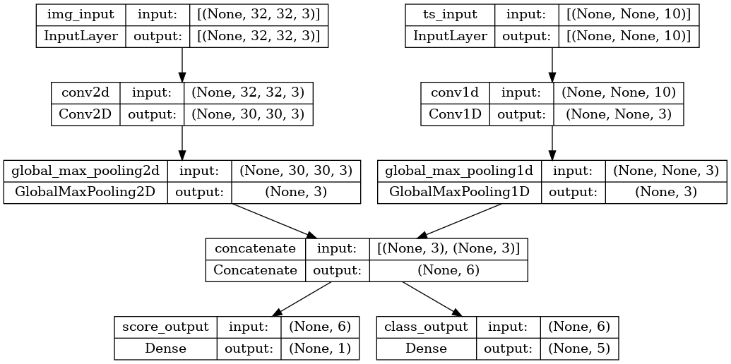
형상 (32, 32, 3)(즉, (height, width, channels))의 이미지 입력과 형상 (None, 10)(즉, (timesteps, features))의 시계열 입력이 있는 다음 모델을 고려해 보겠습니다. 이 모델은 이러한 입력의 조합으로부터 계산된 다음의 두 출력을 가질 것입니다. "score"(형상 (1,)) 및 다섯 개의 클래스에 걸친 확률 분포(형상 (5,))
image_input = keras.Input(shape=(32, 32, 3), name="img_input")
timeseries_input = keras.Input(shape=(None, 10), name="ts_input")

x1 = layers.Conv2D(3, 3)(image_input)
x1 = layers.GlobalMaxPooling2D()(x1)

x2 = layers.Conv1D(3, 3)(timeseries_input)
x2 = layers.GlobalMaxPooling1D()(x2)

x = layers.concatenate([x1, x2])

score_output = layers.Dense(1, name="score_output")(x)
class_output = layers.Dense(5, name="class_output")(x)

model = keras.Model(
    inputs=[image_input, timeseries_input], outputs=[score_output, class_output]
)
이 모델을 플롯해 보면 여기서 수행 중인 작업을 명확하게 확인할 수 있습니다(플롯에 표시된 형상이 샘플별 형상이 아니라 배치 형상임에 주목).
keras.utils.plot_model(model, "multi_input_and_output_model.png", show_shapes=True)
컴파일할 때 손실 함수를 목록으로 전달하여 출력마다 다른 손실을 지정할 수 있습니다.
model.compile(
    optimizer=keras.optimizers.RMSprop(1e-3),
    loss=[keras.losses.MeanSquaredError(), keras.losses.CategoricalCrossentropy()],
)
모델에 단일 손실 함수만 전달하는 경우, 모든 출력에 동일한 손실 함수가 적용됩니다(여기서는 적합하지 않음).
메트릭의 경우도 마찬가지입니다.
model.compile(
    optimizer=keras.optimizers.RMSprop(1e-3),
    loss=[keras.losses.MeanSquaredError(), keras.losses.CategoricalCrossentropy()],
    metrics=[
        [
            keras.metrics.MeanAbsolutePercentageError(),
            keras.metrics.MeanAbsoluteError(),
        ],
        [keras.metrics.CategoricalAccuracy()],
    ],
)
출력 레이어에 이름을 지정했으므로 사전을 통해 출력별 손실과 메트릭을 지정할 수도 있습니다.
model.compile(
    optimizer=keras.optimizers.RMSprop(1e-3),
    loss={
        "score_output": keras.losses.MeanSquaredError(),
        "class_output": keras.losses.CategoricalCrossentropy(),
    },
    metrics={
        "score_output": [
            keras.metrics.MeanAbsolutePercentageError(),
            keras.metrics.MeanAbsoluteError(),
        ],
        "class_output": [keras.metrics.CategoricalAccuracy()],
    },
)
출력이 두 개 이상인 경우 명시적 이름과 사전을 사용하는 것이 좋습니다.
loss_weights 인수를 사용하여 출력별 손실에 서로 다른 가중치를 부여할 수 있습니다(예를 들어, 클래스 손실에 2x의 중요도를 부여하여 이 예에서 "score" 손실에 우선권을 줄 수 있음).
model.compile(
    optimizer=keras.optimizers.RMSprop(1e-3),
    loss={
        "score_output": keras.losses.MeanSquaredError(),
        "class_output": keras.losses.CategoricalCrossentropy(),
    },
    metrics={
        "score_output": [
            keras.metrics.MeanAbsolutePercentageError(),
            keras.metrics.MeanAbsoluteError(),
        ],
        "class_output": [keras.metrics.CategoricalAccuracy()],
    },
    loss_weights={"score_output": 2.0, "class_output": 1.0},
)
이러한 출력이 예측를 위한 것이고 훈련과는 관계가 없는 경우, 특정 출력에 대한 손실을 계산하지 않도록 선택할 수도 있습니다.
# List loss version
model.compile(
    optimizer=keras.optimizers.RMSprop(1e-3),
    loss=[None, keras.losses.CategoricalCrossentropy()],
)

# Or dict loss version
model.compile(
    optimizer=keras.optimizers.RMSprop(1e-3),
    loss={"class_output": keras.losses.CategoricalCrossentropy()},
)
fit()에서 다중 입력 또는 다중 출력 모델로 데이터를 전달하는 것은 컴파일에서 손실 함수를 지정하는 것과 유사한 방식으로 작동합니다. 즉, NumPy 배열 목록(손실 함수를 수신한 출력에 1:1 매핑) 또는 출력 이름을 NumPy 배열에 매핑한 사전을 전달할 수 있습니다.
model.compile(
    optimizer=keras.optimizers.RMSprop(1e-3),
    loss=[keras.losses.MeanSquaredError(), keras.losses.CategoricalCrossentropy()],
)

# Generate dummy NumPy data
img_data = np.random.random_sample(size=(100, 32, 32, 3))
ts_data = np.random.random_sample(size=(100, 20, 10))
score_targets = np.random.random_sample(size=(100, 1))
class_targets = np.random.random_sample(size=(100, 5))

# Fit on lists
model.fit([img_data, ts_data], [score_targets, class_targets], batch_size=32, epochs=1)

# Alternatively, fit on dicts
model.fit(
    {"img_input": img_data, "ts_input": ts_data},
    {"score_output": score_targets, "class_output": class_targets},
    batch_size=32,
    epochs=1,
)
4/4 [==============================] - 2s 10ms/step - loss: 12.6268 - score_output_loss: 0.1838 - class_output_loss: 12.4430
4/4 [==============================] - 0s 5ms/step - loss: 11.8610 - score_output_loss: 0.1694 - class_output_loss: 11.6916
<keras.callbacks.History at 0x7ff5398ecd60>
다음은 Dataset를 사용한 예입니다. NumPy 배열에서 수행한 작업과 유사하게 Dataset은 사전 튜플을 반환해야 합니다.
train_dataset = tf.data.Dataset.from_tensor_slices(
    (
        {"img_input": img_data, "ts_input": ts_data},
        {"score_output": score_targets, "class_output": class_targets},
    )
)
train_dataset = train_dataset.shuffle(buffer_size=1024).batch(64)

model.fit(train_dataset, epochs=1)
2/2 [==============================] - 0s 19ms/step - loss: 11.3569 - score_output_loss: 0.1599 - class_output_loss: 11.1969
<keras.callbacks.History at 0x7ff3ac22c640>
콜백 사용하기
Keras의 콜백은 훈련 중 다른 시점(epoch의 시작, 배치의 끝, epoch의 끝 등)에서 호출되며 다음과 같은 특정 동작을 구현하는 데 사용할 수 있는 객체입니다.
- 훈련 중 서로 다른 시점에서 유효성 검사 수행(내장된 epoch당 유효성 검사에서 더욱 확장)
- 정기적으로 또는 특정 정확도 임계값을 초과할 때 모델 검사점 설정
- 훈련이 평탄해진 것으로 보일 때 모델의 학습률 변경
- 훈련이 평탄해진 것으로 보일 때 최상위 레이어의 미세 조정 수행
- 훈련이 종료되거나 특정 성능 임계값이 초과된 경우 이메일 또는 인스턴트 메시지로 알림 보내기
- 기타
콜백은 fit()에 대한 호출에 목록으로 전달할 수 있습니다.
model = get_compiled_model()

callbacks = [
    keras.callbacks.EarlyStopping(
        # Stop training when `val_loss` is no longer improving
        monitor="val_loss",
        # "no longer improving" being defined as "no better than 1e-2 less"
        min_delta=1e-2,
        # "no longer improving" being further defined as "for at least 2 epochs"
        patience=2,
        verbose=1,
    )
]
model.fit(
    x_train,
    y_train,
    epochs=20,
    batch_size=64,
    callbacks=callbacks,
    validation_split=0.2,
)
Epoch 1/20
625/625 [==============================] - 3s 3ms/step - loss: 0.3826 - sparse_categorical_accuracy: 0.8929 - val_loss: 0.2449 - val_sparse_categorical_accuracy: 0.9290
Epoch 2/20
625/625 [==============================] - 2s 2ms/step - loss: 0.1799 - sparse_categorical_accuracy: 0.9481 - val_loss: 0.1885 - val_sparse_categorical_accuracy: 0.9430
Epoch 3/20
625/625 [==============================] - 2s 3ms/step - loss: 0.1293 - sparse_categorical_accuracy: 0.9621 - val_loss: 0.1619 - val_sparse_categorical_accuracy: 0.9525
Epoch 4/20
625/625 [==============================] - 2s 2ms/step - loss: 0.1009 - sparse_categorical_accuracy: 0.9697 - val_loss: 0.1393 - val_sparse_categorical_accuracy: 0.9580
Epoch 5/20
625/625 [==============================] - 2s 2ms/step - loss: 0.0820 - sparse_categorical_accuracy: 0.9758 - val_loss: 0.1437 - val_sparse_categorical_accuracy: 0.9579
Epoch 6/20
625/625 [==============================] - 2s 2ms/step - loss: 0.0691 - sparse_categorical_accuracy: 0.9790 - val_loss: 0.1316 - val_sparse_categorical_accuracy: 0.9631
Epoch 6: early stopping
<keras.callbacks.History at 0x7ff5397c0c70>
많은 내장 콜백을 사용할 수 있습니다
Keras에서 이미 사용할 수 있는 내장 콜백은 다음과 같습니다.
ModelCheckpoint: 주기적으로 모델을 저장합니다.EarlyStopping: 훈련이 더 이상 유효성 검사 메트릭을 개선하지 못하는 경우 훈련을 중단합니다.TensorBoard: TensorBoard에서 시각화할 수 있는 모델 로그를 정기적으로 작성합니다("시각화" 섹션에서 자세히 설명).CSVLogger: 손실 및 메트릭 데이터를 CSV 파일로 스트리밍합니다.- 기타
전체 목록은 콜백 설명서를 참조하세요.
고유한 콜백 작성하기
기본 클래스 keras.callbacks.Callback을 확장하여 사용자 정의 콜백을 작성할 수 있습니다. 콜백은 클래스 속성 self.model을 통해 연관된 모델에 액세스할 수 있습니다.
사용자 정의 콜백을 작성하기 위한 전체 가이드를 꼭 읽어보세요.
다음은 훈련 중 배치별 손실 값 목록을 저장하는 간단한 예입니다.
class LossHistory(keras.callbacks.Callback):
    def on_train_begin(self, logs):
        self.per_batch_losses = []

    def on_batch_end(self, batch, logs):
        self.per_batch_losses.append(logs.get("loss"))
모델 검사점 설정하기
상대적으로 큰 데이터세트에 대한 모델을 훈련시킬 때는 모델의 검사점을 빈번하게 저장하는 것이 중요합니다.
이를 수행하는 가장 쉬운 방법은 ModelCheckpoint 콜백을 사용하는 것입니다.
model = get_compiled_model()

callbacks = [
    keras.callbacks.ModelCheckpoint(
        # Path where to save the model
        # The two parameters below mean that we will overwrite
        # the current checkpoint if and only if
        # the `val_loss` score has improved.
        # The saved model name will include the current epoch.
        filepath="mymodel_{epoch}",
        save_best_only=True,  # Only save a model if `val_loss` has improved.
        monitor="val_loss",
        verbose=1,
    )
]
model.fit(
    x_train, y_train, epochs=2, batch_size=64, callbacks=callbacks, validation_split=0.2
)
Epoch 1/2
615/625 [============================>.] - ETA: 0s - loss: 0.3780 - sparse_categorical_accuracy: 0.8910
Epoch 1: val_loss improved from inf to 0.23306, saving model to mymodel_1
INFO:tensorflow:Assets written to: mymodel_1/assets
625/625 [==============================] - 3s 4ms/step - loss: 0.3760 - sparse_categorical_accuracy: 0.8917 - val_loss: 0.2331 - val_sparse_categorical_accuracy: 0.9302
Epoch 2/2
614/625 [============================>.] - ETA: 0s - loss: 0.1762 - sparse_categorical_accuracy: 0.9473
Epoch 2: val_loss improved from 0.23306 to 0.17272, saving model to mymodel_2
INFO:tensorflow:Assets written to: mymodel_2/assets
625/625 [==============================] - 2s 3ms/step - loss: 0.1762 - sparse_categorical_accuracy: 0.9474 - val_loss: 0.1727 - val_sparse_categorical_accuracy: 0.9490
<keras.callbacks.History at 0x7ff47c12ef10>
ModelCheckpoint 콜백을 사용하여 내결함성을 구현할 수 있습니다. 즉, 훈련이 무작위로 중단되는 경우 모델의 마지막 저장된 상태에서 훈련을 다시 시작할 수 있습니다. 다음은 기본적인 예입니다.
import os

# Prepare a directory to store all the checkpoints.
checkpoint_dir = "./ckpt"
if not os.path.exists(checkpoint_dir):
    os.makedirs(checkpoint_dir)


def make_or_restore_model():
    # Either restore the latest model, or create a fresh one
    # if there is no checkpoint available.
    checkpoints = [checkpoint_dir + "/" + name for name in os.listdir(checkpoint_dir)]
    if checkpoints:
        latest_checkpoint = max(checkpoints, key=os.path.getctime)
        print("Restoring from", latest_checkpoint)
        return keras.models.load_model(latest_checkpoint)
    print("Creating a new model")
    return get_compiled_model()


model = make_or_restore_model()
callbacks = [
    # This callback saves a SavedModel every 100 batches.
    # We include the training loss in the saved model name.
    keras.callbacks.ModelCheckpoint(
        filepath=checkpoint_dir + "/ckpt-loss={loss:.2f}", save_freq=100
    )
]
model.fit(x_train, y_train, epochs=1, callbacks=callbacks)
Creating a new model
  92/1563 [>.............................] - ETA: 3s - loss: 1.0208 - sparse_categorical_accuracy: 0.7201INFO:tensorflow:Assets written to: ./ckpt/ckpt-loss=0.98/assets
 191/1563 [==>...........................] - ETA: 6s - loss: 0.7268 - sparse_categorical_accuracy: 0.7999INFO:tensorflow:Assets written to: ./ckpt/ckpt-loss=0.71/assets
 291/1563 [====>.........................] - ETA: 6s - loss: 0.5989 - sparse_categorical_accuracy: 0.8316INFO:tensorflow:Assets written to: ./ckpt/ckpt-loss=0.59/assets
 394/1563 [======>.......................] - ETA: 6s - loss: 0.5316 - sparse_categorical_accuracy: 0.8505INFO:tensorflow:Assets written to: ./ckpt/ckpt-loss=0.53/assets
 495/1563 [========>.....................] - ETA: 6s - loss: 0.4830 - sparse_categorical_accuracy: 0.8626INFO:tensorflow:Assets written to: ./ckpt/ckpt-loss=0.48/assets
 591/1563 [==========>...................] - ETA: 5s - loss: 0.4490 - sparse_categorical_accuracy: 0.8720INFO:tensorflow:Assets written to: ./ckpt/ckpt-loss=0.45/assets
 693/1563 [============>.................] - ETA: 5s - loss: 0.4219 - sparse_categorical_accuracy: 0.8789INFO:tensorflow:Assets written to: ./ckpt/ckpt-loss=0.42/assets
 791/1563 [==============>...............] - ETA: 4s - loss: 0.4002 - sparse_categorical_accuracy: 0.8848INFO:tensorflow:Assets written to: ./ckpt/ckpt-loss=0.40/assets
 892/1563 [================>.............] - ETA: 4s - loss: 0.3852 - sparse_categorical_accuracy: 0.8888INFO:tensorflow:Assets written to: ./ckpt/ckpt-loss=0.38/assets
 991/1563 [==================>...........] - ETA: 3s - loss: 0.3685 - sparse_categorical_accuracy: 0.8934INFO:tensorflow:Assets written to: ./ckpt/ckpt-loss=0.37/assets
1091/1563 [===================>..........] - ETA: 2s - loss: 0.3543 - sparse_categorical_accuracy: 0.8974INFO:tensorflow:Assets written to: ./ckpt/ckpt-loss=0.35/assets
1189/1563 [=====================>........] - ETA: 2s - loss: 0.3433 - sparse_categorical_accuracy: 0.9007INFO:tensorflow:Assets written to: ./ckpt/ckpt-loss=0.34/assets
1291/1563 [=======================>......] - ETA: 1s - loss: 0.3312 - sparse_categorical_accuracy: 0.9041INFO:tensorflow:Assets written to: ./ckpt/ckpt-loss=0.33/assets
1390/1563 [=========================>....] - ETA: 1s - loss: 0.3221 - sparse_categorical_accuracy: 0.9068INFO:tensorflow:Assets written to: ./ckpt/ckpt-loss=0.32/assets
1491/1563 [===========================>..] - ETA: 0s - loss: 0.3130 - sparse_categorical_accuracy: 0.9094INFO:tensorflow:Assets written to: ./ckpt/ckpt-loss=0.31/assets
1563/1563 [==============================] - 11s 6ms/step - loss: 0.3085 - sparse_categorical_accuracy: 0.9107
<keras.callbacks.History at 0x7ff3ac721910>
모델 저장 및 복원을 위한 자체 콜백을 작성할 수도 있습니다.
직렬화 및 저장에 대한 자세한 설명은 모델 저장 및 직렬화 가이드를 참조하세요.
학습률 일정 사용하기
딥 러닝 모델을 훈련할 때 일반적인 패턴은 훈련이 진행됨에 따라 점차적으로 학습을 줄이는 것입니다. 이것을 일반적으로 "학습률 감소"라고 합니다.
학습 감소 일정은 정적(현재 epoch 또는 현재 배치 인덱스의 함수로 미리 고정됨) 또는 동적(모델의 현재 동작, 특히 유효성 검사 손실에 대응)일 수 있습니다.
최적화 프로그램으로 일정 전달하기
최적화 프로그램에서 schedule 객체를 learning_rate 인수로 전달하여 정적 학습률 감소 일정을 쉽게 사용할 수 있습니다.
initial_learning_rate = 0.1
lr_schedule = keras.optimizers.schedules.ExponentialDecay(
    initial_learning_rate, decay_steps=100000, decay_rate=0.96, staircase=True
)

optimizer = keras.optimizers.RMSprop(learning_rate=lr_schedule)
ExponentialDecay , PiecewiseConstantDecay , PolynomialDecay 및 InverseTimeDecay와 같은 몇 가지 내장된 일정을 사용할 수 있습니다.
콜백을 사용하여 동적 학습률 일정 구현하기
최적화 프로그램이 유효성 검사 메트릭에 액세스할 수 없으므로 이러한 일정 객체로는 동적 학습률 일정(예: 유효성 검사 손실이 더 이상 개선되지 않을 때 학습률 감소)을 달성할 수 없습니다.
그러나 콜백은 유효성 검사 메트릭을 포함해 모든 메트릭에 액세스할 수 있습니다! 따라서 최적화 프로그램에서 현재 학습률을 수정하는 콜백을 사용하여 이 패턴을 달성할 수 있습니다. 실제로 이 부분이ReduceLROnPlateau 콜백으로 내장되어 있습니다.
훈련 중 손실 및 메트릭 시각화하기
훈련 중에 모델을 주시하는 가장 좋은 방법은 로컬에서 실행할 수 있는 브라우저 기반 애플리케이션인 TensorBoard를 사용하는 것입니다. 이 보드에는 다음과 같은 정보가 제공됩니다.
- 훈련 및 평가를 위한 손실 및 메트릭을 실시간으로 플롯
- (옵션) 레이어 활성화 히스토그램 시각화
- (옵션)
Embedding레이어에서 학습한 포함된 공간의 3D 시각화
pip와 함께 TensorFlow를 설치한 경우, 명령줄에서 TensorBoard를 시작할 수 있습니다.
tensorboard --logdir=/full_path_to_your_logs
TensorBoard 콜백 사용하기
TensorBoard를 Keras 모델 및 fit() 메서드와 함께 사용하는 가장 쉬운 방법은 TensorBoard 콜백입니다.
가장 간단한 경우로, 콜백에서 로그를 작성할 위치만 지정하면 바로 로그를 작성할 수 있습니다.
keras.callbacks.TensorBoard(
    log_dir="/full_path_to_your_logs",
    histogram_freq=0,  # How often to log histogram visualizations
    embeddings_freq=0,  # How often to log embedding visualizations
    update_freq="epoch",
)  # How often to write logs (default: once per epoch)
<keras.callbacks.TensorBoard at 0x7ff3ac42bbe0>
자세한 정보는 TensorBoard 콜백 설명서를 참조하세요.