
|
|
|
 View source on GitHub View source on GitHub
|
|
In this colab we'll explore sampling from the posterior of a Bayesian Gaussian Mixture Model (BGMM) using only TensorFlow Probability primitives.
Model
For \(k\in\{1,\ldots, K\}\) mixture components each of dimension \(D\), we'd like to model \(i\in\{1,\ldots,N\}\) iid samples using the following Bayesian Gaussian Mixture Model:
\[\begin{align*} \theta &\sim \text{Dirichlet}(\text{concentration}=\alpha_0)\\ \mu_k &\sim \text{Normal}(\text{loc}=\mu_{0k}, \text{scale}=I_D)\\ T_k &\sim \text{Wishart}(\text{df}=5, \text{scale}=I_D)\\ Z_i &\sim \text{Categorical}(\text{probs}=\theta)\\ Y_i &\sim \text{Normal}(\text{loc}=\mu_{z_i}, \text{scale}=T_{z_i}^{-1/2})\\ \end{align*}\]
Note, the scale arguments all have cholesky semantics. We use this convention because it is that of TF Distributions (which itself uses this convention in part because it is computationally advantageous).
Our goal is to generate samples from the posterior:
\[p\left(\theta, \{\mu_k, T_k\}_{k=1}^K \Big| \{y_i\}_{i=1}^N, \alpha_0, \{\mu_{ok}\}_{k=1}^K\right)\]
Notice that \(\{Z_i\}_{i=1}^N\) is not present--we're interested in only those random variables which don't scale with \(N\). (And luckily there's a TF distribution which handles marginalizing out \(Z_i\).)
It is not possible to directly sample from this distribution owing to a computationally intractable normalization term.
Metropolis-Hastings algorithms are techniques for sampling from intractable-to-normalize distributions.
TensorFlow Probability offers a number of MCMC options, including several based on Metropolis-Hastings. In this notebook, we'll use Hamiltonian Monte Carlo (tfp.mcmc.HamiltonianMonteCarlo). HMC is often a good choice because it can converge rapidly, samples the state space jointly (as opposed to coordinatewise), and leverages one of TF's virtues: automatic differentiation. That said, sampling from a BGMM posterior might actually be better done by other approaches, e.g., Gibb's sampling.
%matplotlib inline


import functools

import matplotlib.pyplot as plt; plt.style.use('ggplot')
import numpy as np
import seaborn as sns; sns.set_context('notebook')

import tensorflow.compat.v2 as tf
tf.enable_v2_behavior()
import tensorflow_probability as tfp

tfd = tfp.distributions
tfb = tfp.bijectors

physical_devices = tf.config.experimental.list_physical_devices('GPU')
if len(physical_devices) > 0:
  tf.config.experimental.set_memory_growth(physical_devices[0], True)
Before actually building the model, we'll need to define a new type of distribution. From the model specification above, it's clear we're parameterizing the MVN with an inverse covariance matrix, i.e., [precision matrix](https://en.wikipedia.org/wiki/Precision_(statistics%29). To accomplish this in TF, we'll need to roll out our Bijector. This Bijector will use the forward transformation:
Y = tf.linalg.triangular_solve((tf.linalg.matrix_transpose(chol_precision_tril), X, adjoint=True) + loc.
And the log_prob calculation is just the inverse, i.e.:
X = tf.linalg.matmul(chol_precision_tril, X - loc, adjoint_a=True).
Since all we need for HMC is log_prob, this means we avoid ever calling tf.linalg.triangular_solve (as would be the case for tfd.MultivariateNormalTriL). This is advantageous since tf.linalg.matmul is usually faster owing to better cache locality.
class MVNCholPrecisionTriL(tfd.TransformedDistribution):
  """MVN from loc and (Cholesky) precision matrix."""

  def __init__(self, loc, chol_precision_tril, name=None):
    super(MVNCholPrecisionTriL, self).__init__(
        distribution=tfd.Independent(tfd.Normal(tf.zeros_like(loc),
                                                scale=tf.ones_like(loc)),
                                     reinterpreted_batch_ndims=1),
        bijector=tfb.Chain([
            tfb.Shift(shift=loc),
            tfb.Invert(tfb.ScaleMatvecTriL(scale_tril=chol_precision_tril,
                                           adjoint=True)),
        ]),
        name=name)
The tfd.Independent distribution turns independent draws of one distribution, into a multivariate distribution with statistically independent coordinates. In terms of computing log_prob, this "meta-distribution" manifests as a simple sum over the event dimension(s).
Also notice that we took the adjoint ("transpose") of the scale matrix. This is because if precision is inverse covariance, i.e., \(P=C^{-1}\) and if \(C=AA^\top\), then \(P=BB^{\top}\) where \(B=A^{-\top}\).
Since this distribution is kind of tricky, let's quickly verify that our MVNCholPrecisionTriL works as we think it should.
def compute_sample_stats(d, seed=42, n=int(1e6)):
  x = d.sample(n, seed=seed)
  sample_mean = tf.reduce_mean(x, axis=0, keepdims=True)
  s = x - sample_mean
  sample_cov = tf.linalg.matmul(s, s, adjoint_a=True) / tf.cast(n, s.dtype)
  sample_scale = tf.linalg.cholesky(sample_cov)
  sample_mean = sample_mean[0]
  return [
      sample_mean,
      sample_cov,
      sample_scale,
  ]

dtype = np.float32
true_loc = np.array([1., -1.], dtype=dtype)
true_chol_precision = np.array([[1., 0.],
                                [2., 8.]],
                               dtype=dtype)
true_precision = np.matmul(true_chol_precision, true_chol_precision.T)
true_cov = np.linalg.inv(true_precision)

d = MVNCholPrecisionTriL(
    loc=true_loc,
    chol_precision_tril=true_chol_precision)

[sample_mean, sample_cov, sample_scale] = [
    t.numpy() for t in compute_sample_stats(d)]

print('true mean:', true_loc)
print('sample mean:', sample_mean)
print('true cov:\n', true_cov)
print('sample cov:\n', sample_cov)
true mean: [ 1. -1.]
sample mean: [ 1.0002806 -1.000105 ]
true cov:
 [[ 1.0625   -0.03125 ]
 [-0.03125   0.015625]]
sample cov:
 [[ 1.0641273  -0.03126175]
 [-0.03126175  0.01559312]]
Since the sample mean and covariance are close to the true mean and covariance, it seems like the distribution is correctly implemented. Now, we'll use MVNCholPrecisionTriL tfp.distributions.JointDistributionNamed to specify the BGMM model. For the observational model, we'll use tfd.MixtureSameFamily to automatically integrate out the \(\{Z_i\}_{i=1}^N\) draws.
dtype = np.float64
dims = 2
components = 3
num_samples = 1000
bgmm = tfd.JointDistributionNamed(dict(
  mix_probs=tfd.Dirichlet(
    concentration=np.ones(components, dtype) / 10.),
  loc=tfd.Independent(
    tfd.Normal(
        loc=np.stack([
            -np.ones(dims, dtype),
            np.zeros(dims, dtype),
            np.ones(dims, dtype),
        ]),
        scale=tf.ones([components, dims], dtype)),
    reinterpreted_batch_ndims=2),
  precision=tfd.Independent(
    tfd.WishartTriL(
        df=5,
        scale_tril=np.stack([np.eye(dims, dtype=dtype)]*components),
        input_output_cholesky=True),
    reinterpreted_batch_ndims=1),
  s=lambda mix_probs, loc, precision: tfd.Sample(tfd.MixtureSameFamily(
      mixture_distribution=tfd.Categorical(probs=mix_probs),
      components_distribution=MVNCholPrecisionTriL(
          loc=loc,
          chol_precision_tril=precision)),
      sample_shape=num_samples)
))
def joint_log_prob(observations, mix_probs, loc, chol_precision):
  """BGMM with priors: loc=Normal, precision=Inverse-Wishart, mix=Dirichlet.

  Args:
    observations: `[n, d]`-shaped `Tensor` representing Bayesian Gaussian
      Mixture model draws. Each sample is a length-`d` vector.
    mix_probs: `[K]`-shaped `Tensor` representing random draw from
      `Dirichlet` prior.
    loc: `[K, d]`-shaped `Tensor` representing the location parameter of the
      `K` components.
    chol_precision: `[K, d, d]`-shaped `Tensor` representing `K` lower
      triangular `cholesky(Precision)` matrices, each being sampled from
      a Wishart distribution.

  Returns:
    log_prob: `Tensor` representing joint log-density over all inputs.
  """
  return bgmm.log_prob(
      mix_probs=mix_probs, loc=loc, precision=chol_precision, s=observations)
Generate "Training" Data
For this demo, we'll sample some random data.
true_loc = np.array([[-2., -2],
                     [0, 0],
                     [2, 2]], dtype)
random = np.random.RandomState(seed=43)

true_hidden_component = random.randint(0, components, num_samples)
observations = (true_loc[true_hidden_component] +
                random.randn(num_samples, dims).astype(dtype))
Bayesian Inference using HMC
Now that we've used TFD to specify our model and obtained some observed data, we have all the necessary pieces to run HMC.
To do this, we'll use a partial application to "pin down" the things we don't want to sample. In this case that means we need only pin down observations. (The hyper-parameters are already baked in to the prior distributions and not part of the joint_log_prob function signature.)
unnormalized_posterior_log_prob = functools.partial(joint_log_prob, observations)
initial_state = [
    tf.fill([components],
            value=np.array(1. / components, dtype),
            name='mix_probs'),
    tf.constant(np.array([[-2., -2],
                          [0, 0],
                          [2, 2]], dtype),
                name='loc'),
    tf.linalg.eye(dims, batch_shape=[components], dtype=dtype, name='chol_precision'),
]
Unconstrained Representation
Hamiltonian Monte Carlo (HMC) requires the target log-probability function to be differentiable with respect to its arguments. Furthermore, HMC can exhibit dramatically higher statistical efficiency if the state-space is unconstrained.
This means we'll have to work out two main issues when sampling from the BGMM posterior:
- \(\theta\) represents a discrete probability vector, i.e., must be such that \(\sum_{k=1}^K \theta_k = 1\) and \(\theta_k>0\).
- \(T_k\) represents an inverse covariance matrix, i.e., must be such that \(T_k \succ 0\), i.e., is positive definite.
To address this requirement we'll need to:
- transform the constrained variables to an unconstrained space
- run the MCMC in unconstrained space
- transform the unconstrained variables back to the constrained space.
As with MVNCholPrecisionTriL, we'll use Bijectors to transform random variables to unconstrained space.
The
Dirichletis transformed to unconstrained space via the softmax function.Our precision random variable is a distribution over positive semidefinite matrices. To unconstrain these we'll use the
FillTriangularandTransformDiagonalbijectors. These convert vectors to lower-triangular matrices and ensure the diagonal is positive. The former is useful because it enables sampling only \(d(d+1)/2\) floats rather than \(d^2\).
unconstraining_bijectors = [
    tfb.SoftmaxCentered(),
    tfb.Identity(),
    tfb.Chain([
        tfb.TransformDiagonal(tfb.Softplus()),
        tfb.FillTriangular(),
    ])]
@tf.function(autograph=False)
def sample():
  return tfp.mcmc.sample_chain(
    num_results=2000,
    num_burnin_steps=500,
    current_state=initial_state,
    kernel=tfp.mcmc.SimpleStepSizeAdaptation(
        tfp.mcmc.TransformedTransitionKernel(
            inner_kernel=tfp.mcmc.HamiltonianMonteCarlo(
                target_log_prob_fn=unnormalized_posterior_log_prob,
                 step_size=0.065,
                 num_leapfrog_steps=5),
            bijector=unconstraining_bijectors),
         num_adaptation_steps=400),
    trace_fn=lambda _, pkr: pkr.inner_results.inner_results.is_accepted)

[mix_probs, loc, chol_precision], is_accepted = sample()
We'll now execute the chain and print the posterior means.
acceptance_rate = tf.reduce_mean(tf.cast(is_accepted, dtype=tf.float32)).numpy()
mean_mix_probs = tf.reduce_mean(mix_probs, axis=0).numpy()
mean_loc = tf.reduce_mean(loc, axis=0).numpy()
mean_chol_precision = tf.reduce_mean(chol_precision, axis=0).numpy()
precision = tf.linalg.matmul(chol_precision, chol_precision, transpose_b=True)
print('acceptance_rate:', acceptance_rate)
print('avg mix probs:', mean_mix_probs)
print('avg loc:\n', mean_loc)
print('avg chol(precision):\n', mean_chol_precision)
acceptance_rate: 0.5305
avg mix probs: [0.25248723 0.60729516 0.1402176 ]
avg loc:
 [[-1.96466753 -2.12047249]
 [ 0.27628865  0.22944732]
 [ 2.06461244  2.54216122]]
avg chol(precision):
 [[[ 1.05105032  0.        ]
  [ 0.12699955  1.06553113]]

 [[ 0.76058015  0.        ]
  [-0.50332767  0.77947431]]

 [[ 1.22770457  0.        ]
  [ 0.70670027  1.50914164]]]
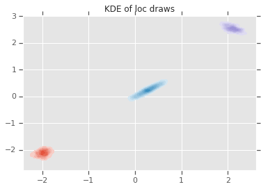
loc_ = loc.numpy()
ax = sns.kdeplot(loc_[:,0,0], loc_[:,0,1], shade=True, shade_lowest=False)
ax = sns.kdeplot(loc_[:,1,0], loc_[:,1,1], shade=True, shade_lowest=False)
ax = sns.kdeplot(loc_[:,2,0], loc_[:,2,1], shade=True, shade_lowest=False)
plt.title('KDE of loc draws');
Conclusion
This simple colab demonstrated how TensorFlow Probability primitives can be used to build hierarchical Bayesian mixture models.