
| |
|
 在 Github 上查看源代码 在 Github 上查看源代码 |
|
import numpy as np
import matplotlib.pyplot as plt
import tensorflow.compat.v2 as tf
tf.enable_v2_behavior()

import tensorflow_probability as tfp
tfd = tfp.distributions
tfb = tfp.bijectors
[Copula](https://en.wikipedia.org/wiki/Copula_(probability_theory%29) 是一种捕获随机变量之间依赖关系的经典方式。更正式地说,Copula 是一种多元分布 \(C(U_1, U_2, ...., U_n)\),通过边缘化得到 \(U_i \sim \text{Uniform}(0, 1)\)。
Copula 很有趣,因为我们可以用它来创建任意边缘的多元分布。配方如下:
- 使用概率积分变换将任意连续的 R.V. \(X\) 变为一个均匀的 \(F_X(X)\),其中 \(F_X\) 是 \(X\) 的 CDF。
- 给定一个 Copula(比如,二元变量)\(C(U, V)\),我们会得到 \(U\) 和 \(V\) 具有均匀的边缘分布。
- 现在给定我们感兴趣的 R.V's \(X, Y\),创建一个新的分布 \(C'(X, Y) = C(F_X(X), F_Y(Y))\)。\(X\) 和 \(Y\) 的边缘是我们想要的。
边缘是单变量的,因此可能更容易测量和/或建模。Copula 可以从边缘开始,但也可以实现各维度之间的任意关联。
高斯 Copula
为了说明如何构造 Copula,请考虑根据多元高斯相关性来捕获依赖关系的情况。高斯 Copula 由 \(C(u_1, u_2, ...u_n) = \Phi_\Sigma(\Phi^{-1}(u_1), \Phi^{-1}(u_2), ... \Phi^{-1}(u_n))\) 给出,其中 \(\Phi_\Sigma\) 表示多元正态分布的 CDF,协方差为 \(\Sigma\),均值为 0,\(\Phi^{-1}\) 是标准正态分布的逆 CDF。
应用正态分布的逆 CDF 会将均匀维度扭曲为正态分布。应用多元正态分布的 CDF 则会将分布挤压为边缘均匀且具有高斯相关性。
因此,我们得到的高斯 Copula 是在单位超立方体 \([0, 1]^n\) 上具有均匀边缘的分布。
这样定义的高斯 Copula 可以使用 tfd.TransformedDistribution 和适当的 Bijector 来实现。也就是说,我们通过使用正态分布的逆 CDF(由 tfb.NormalCDF 双射器实现)来变换多元正态分布。
下面,我们用一个简化的假设来实现高斯 Copula:协方差由 Cholesky 因子参数化(因此为 MultivariateNormalTriL 的协方差)。(我们可以使用其他 tf.linalg.LinearOperators 来编码不同的无矩阵假设)。
class GaussianCopulaTriL(tfd.TransformedDistribution):
"""Takes a location, and lower triangular matrix for the Cholesky factor."""
def __init__(self, loc, scale_tril):
super(GaussianCopulaTriL, self).__init__(
distribution=tfd.MultivariateNormalTriL(
loc=loc,
scale_tril=scale_tril),
bijector=tfb.NormalCDF(),
validate_args=False,
name="GaussianCopulaTriLUniform")
# Plot an example of this.
unit_interval = np.linspace(0.01, 0.99, num=200, dtype=np.float32)
x_grid, y_grid = np.meshgrid(unit_interval, unit_interval)
coordinates = np.concatenate(
[x_grid[..., np.newaxis],
y_grid[..., np.newaxis]], axis=-1)
pdf = GaussianCopulaTriL(
loc=[0., 0.],
scale_tril=[[1., 0.8], [0., 0.6]],
).prob(coordinates)
# Plot its density.
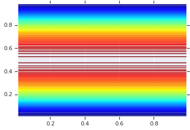
plt.contour(x_grid, y_grid, pdf, 100, cmap=plt.cm.jet);
然而,这种模型的功效在于使用概率积分变换,以在任意 R.V.s. 上使用 Copula。这样,我们可以指定任意边缘,并使用 Copula 将它们拼接在一起。
我们从下面的模型开始:
\[\begin{align*} X &\sim \text{Kumaraswamy}(a, b) \ Y &\sim \text{Gumbel}(\mu, \beta) \end{align*}\]
使用 Copula 获得一个双变量 R.V. \(Z\),其边缘为 Kumaraswamy 和 Gumbel。
我们先绘制由这两个 R.V.s. 生成的积分布。这只是作为我们应用 Copula 时的一个比较点。
a = 2.0
b = 2.0
gloc = 0.
gscale = 1.

x = tfd.Kumaraswamy(a, b)
y = tfd.Gumbel(loc=gloc, scale=gscale)

# Plot the distributions, assuming independence
x_axis_interval = np.linspace(0.01, 0.99, num=200, dtype=np.float32)
y_axis_interval = np.linspace(-2., 3., num=200, dtype=np.float32)
x_grid, y_grid = np.meshgrid(x_axis_interval, y_axis_interval)

pdf = x.prob(x_grid) * y.prob(y_grid)

# Plot its density

plt.contour(x_grid, y_grid, pdf, 100, cmap=plt.cm.jet);
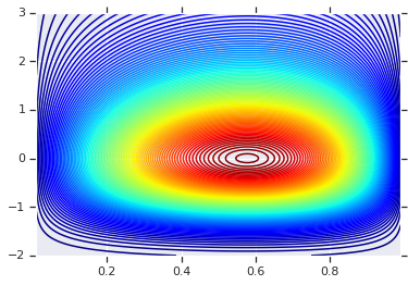
具有不同边缘的联合分布
现在,我们使用高斯 Copula 将分布耦合在一起,并进行绘制。同样,我们选择的工具是 TransformedDistribution,应用适当的 Bijector 来获得所选的边缘。
具体来说,我们使用 Blockwise 双射器,它会在向量的不同部分应用不同的双射器(仍然是双射变换)。
现在,我们可以定义想要的 Copula。给定一个目标边缘的列表(编码为双射器),我们可以轻松构造一个使用 Copula 并具有指定边缘的新分布。
class WarpedGaussianCopula(tfd.TransformedDistribution):
  """Application of a Gaussian Copula on a list of target marginals.

  This implements an application of a Gaussian Copula. Given [x_0, ... x_n]
  which are distributed marginally (with CDF) [F_0, ... F_n],
  `GaussianCopula` represents an application of the Copula, such that the
  resulting multivariate distribution has the above specified marginals.

  The marginals are specified by `marginal_bijectors`: These are
  bijectors whose `inverse` encodes the CDF and `forward` the inverse CDF.

  block_sizes is a 1-D Tensor to determine splits for `marginal_bijectors`
  length should be same as length of `marginal_bijectors`.
  See tfb.Blockwise for details
  """
  def __init__(self, loc, scale_tril, marginal_bijectors, block_sizes=None):
    super(WarpedGaussianCopula, self).__init__(
        distribution=GaussianCopulaTriL(loc=loc, scale_tril=scale_tril),
        bijector=tfb.Blockwise(bijectors=marginal_bijectors,
                               block_sizes=block_sizes),
        validate_args=False,
        name="GaussianCopula")
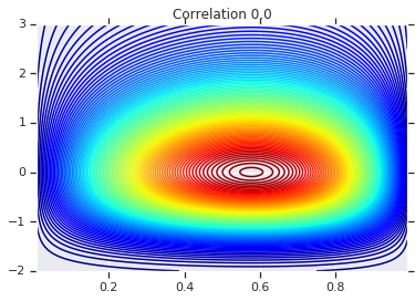
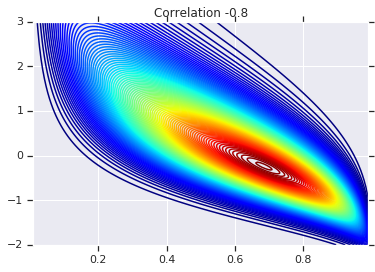
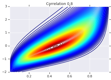
最后,我们来实际使用这个高斯 Copula。我们将使用 \(\begin{bmatrix}1 & 0\rho & \sqrt{(1-\rho^2)}\end{bmatrix}\) 的Cholesky,它将对应于方差 1,以及多元正态分布的相关性 \(\rho\)。
我们来看几种情况:
# Create our coordinates:
coordinates = np.concatenate(
    [x_grid[..., np.newaxis], y_grid[..., np.newaxis]], -1)


def create_gaussian_copula(correlation):
  # Use Gaussian Copula to add dependence.
  return WarpedGaussianCopula(
      loc=[0.,  0.],
      scale_tril=[[1., 0.], [correlation, tf.sqrt(1. - correlation ** 2)]],
      # These encode the marginals we want. In this case we want X_0 has
      # Kumaraswamy marginal, and X_1 has Gumbel marginal.

      marginal_bijectors=[
          tfb.Invert(tfb.KumaraswamyCDF(a, b)),
          tfb.Invert(tfb.GumbelCDF(loc=0., scale=1.))])


# Note that the zero case will correspond to independent marginals!
correlations = [0., -0.8, 0.8]
copulas = []
probs = []
for correlation in correlations:
  copula = create_gaussian_copula(correlation)
  copulas.append(copula)
  probs.append(copula.prob(coordinates))


# Plot it's density

for correlation, copula_prob in zip(correlations, probs):
  plt.figure()
  plt.contour(x_grid, y_grid, copula_prob, 100, cmap=plt.cm.jet)
  plt.title('Correlation {}'.format(correlation))
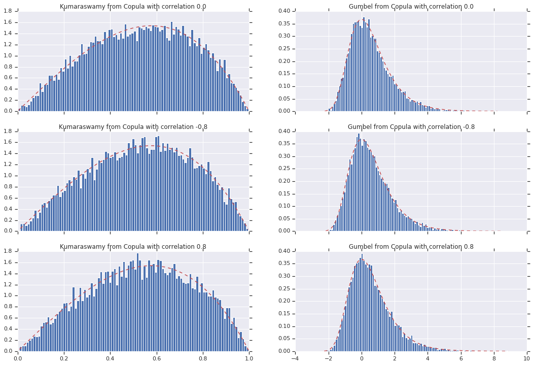
最后,我们来验证一下,我们是否确实获得了所需的边缘。
def kumaraswamy_pdf(x):
    return tfd.Kumaraswamy(a, b).prob(np.float32(x))

def gumbel_pdf(x):
    return tfd.Gumbel(gloc, gscale).prob(np.float32(x))


copula_samples = []
for copula in copulas:
  copula_samples.append(copula.sample(10000))

plot_rows = len(correlations)
plot_cols = 2  # for 2  densities [kumarswamy, gumbel]
fig, axes = plt.subplots(plot_rows, plot_cols, sharex='col', figsize=(18,12))

# Let's marginalize out on each, and plot the samples.

for i, (correlation, copula_sample) in enumerate(zip(correlations, copula_samples)):
  k = copula_sample[..., 0].numpy()
  g = copula_sample[..., 1].numpy()


  _, bins, _ = axes[i, 0].hist(k, bins=100, density=True)
  axes[i, 0].plot(bins, kumaraswamy_pdf(bins), 'r--')
  axes[i, 0].set_title('Kumaraswamy from Copula with correlation {}'.format(correlation))

  _, bins, _ = axes[i, 1].hist(g, bins=100, density=True)
  axes[i, 1].plot(bins, gumbel_pdf(bins), 'r--')
  axes[i, 1].set_title('Gumbel from Copula with correlation {}'.format(correlation))
结论
我们成功了!我们已经证明了可以使用 Bijector API 构造高斯 Copula。
概括地说就是,使用 Bijector API 编写双射器,并将其与分布组合在一起,可以创建丰富的分布系列,实现灵活建模。