변이 추론을 사용하여 일반화 선형 혼합 효과 모델 피팅

TensorFlow.org에서 보기

Google Colab에서 실행

GitHub에서 소스 보기

노트북 다운로드

설치

TF_Installation = 'System'

if TF_Installation == 'TF Nightly':
  !pip install -q --upgrade tf-nightly
  print('Installation of `tf-nightly` complete.')
elif TF_Installation == 'TF Stable':
  !pip install -q --upgrade tensorflow
  print('Installation of `tensorflow` complete.')
elif TF_Installation == 'System':
  pass
else:
  raise ValueError('Selection Error: Please select a valid '
                   'installation option.')

설치

TFP_Installation = "System"

if TFP_Installation == "Nightly":
  !pip install -q tfp-nightly
  print("Installation of `tfp-nightly` complete.")
elif TFP_Installation == "Stable":
  !pip install -q --upgrade tensorflow-probability
  print("Installation of `tensorflow-probability` complete.")
elif TFP_Installation == "System":
  pass
else:
  raise ValueError("Selection Error: Please select a valid "
                   "installation option.")

추상적 인

이 colab에서는 TensorFlow Probability에서 변형 추론을 사용하여 일반화된 선형 혼합 효과 모델을 맞추는 방법을 보여줍니다.

모델 패밀리

혼합 효과 모델 일반화 선형 (GLMM) 유사한 일반화 된 선형 모델 들은 선형 예측에 응답하여 샘플 특정 노이즈를 포함하는 것을 제외하고 (GLM). 이것은 거의 보이지 않는 기능이 더 일반적으로 보이는 기능과 정보를 공유할 수 있도록 하기 때문에 부분적으로 유용합니다.

생성 과정으로서 일반화 선형 혼합 효과 모델(GLMM)은 다음과 같은 특징이 있습니다.

\[ \begin{align} \text{for } & r = 1\ldots R: \hspace{2.45cm}\text{# for each random-effect group}\\ &\begin{aligned} \text{for } &c = 1\ldots |C_r|: \hspace{1.3cm}\text{# for each category ("level") of group $r$}\\ &\begin{aligned} \beta_{rc} &\sim \text{MultivariateNormal}(\text{loc}=0_{D_r}, \text{scale}=\Sigma_r^{1/2}) \end{aligned} \end{aligned}\\\\ \text{for } & i = 1 \ldots N: \hspace{2.45cm}\text{# for each sample}\\ &\begin{aligned} &\eta_i = \underbrace{\vphantom{\sum_{r=1}^R}x_i^\top\omega}_\text{fixed-effects} + \underbrace{\sum_{r=1}^R z_{r,i}^\top \beta_{r,C_r(i) } }_\text{random-effects} \\ &Y_i|x_i,\omega,\{z_{r,i} , \beta_r\}_{r=1}^R \sim \text{Distribution}(\text{mean}= g^{-1}(\eta_i)) \end{aligned} \end{align} \]

어디:

\[ \begin{align} R &= \text{number of random-effect groups}\\ |C_r| &= \text{number of categories for group $r$}\\ N &= \text{number of training samples}\\ x_i,\omega &\in \mathbb{R}^{D_0}\\ D_0 &= \text{number of fixed-effects}\\ C_r(i) &= \text{category (under group $r$) of the $i$th sample}\\ z_{r,i} &\in \mathbb{R}^{D_r}\\ D_r &= \text{number of random-effects associated with group $r$}\\ \Sigma_{r} &\in \{S\in\mathbb{R}^{D_r \times D_r} : S \succ 0 \}\\ \eta_i\mapsto g^{-1}(\eta_i) &= \mu_i, \text{inverse link function}\\ \text{Distribution} &=\text{some distribution parameterizable solely by its mean} \end{align} \]

즉,이 각 그룹의 모든 범주 샘플과 연결되어 있다고 \(\beta_{rc}\)다변량 정상에서. 있지만 \(\beta_{rc}\) 항상 독립적립니다, 그들은 단지 indentically 그룹에 대한 분산 \(r\): 통지가 정확히 하나가 \(\Sigma_r\) 각 \(r\in\{1,\ldots,R\}\).

affinely 샘플의 그룹의 기능 (결합하면\(z_{r,i}\)) 결과는 샘플에서 고유의 잡음 \(i\)(달리 인 선형 응답을 예측 번째 \(x_i^\top\omega\)).

우리가 추정 할 때 \(\{\Sigma_r:r\in\{1,\ldots,R\}\}\) 우리는 본질적으로 다른에 존재하는 신호 익사 것이다 임의 효과 그룹이 수행 잡음의 양을 추정하고 \(x_i^\top\omega\).

에 대한 다양한 옵션이 있습니다 \(\text{Distribution}\) 및 역 링크 기능 , \(g^{-1}\). 일반적인 선택은 다음과 같습니다.

• \(Y_i\sim\text{Normal}(\text{mean}=\eta_i, \text{scale}=\sigma)\),
• \(Y_i\sim\text{Binomial}(\text{mean}=n_i \cdot \text{sigmoid}(\eta_i), \text{total_count}=n_i)\)하고,
• \(Y_i\sim\text{Poisson}(\text{mean}=\exp(\eta_i))\).

더 많은 가능성의 경우, 참조 tfp.glm 모듈을.

변이 추론

불행하게도, 매개 변수의 최대 우도 추정 찾는 \(\beta,\{\Sigma_r\}_r^R\) 수반 비 분석 적분. 이 문제를 피하기 위해 우리는 대신

1. 분포 파라미터 패밀리 (이하 "대리 밀도"), 표시 정의 \(q_{\lambda}\) 부록있다.
2. 매개 변수 찾기 \(\lambda\) 수 있도록 \(q_{\lambda}\) 가까운 우리의 진정한 목표 denstiy이다.

분포의 가정은, 우리의 "최소 의미한다 독립적 적절한 차원 가우시안 및"목표 농도에 근접 "가 될 것이다 쿨백 - 라이 블러 발산을 ". 예를 들어, 참조 : "통계 학자에 대한 리뷰 변분 추론"의 2.2 절 잘 작성 유도 및 동기 부여. 특히 KL divergence를 최소화하는 것이 ELBO(negative evidence lower bound)를 최소화하는 것과 동일함을 보여줍니다.

장난감 문제

겔만 외.의 (2007) "라돈 데이터 세트는" 때때로 회귀에 대한 접근 방법을 설명하는 데 사용되는 데이터 세트입니다. (예,이 밀접하게 관련 PyMC3의 블로그 게시물 .) 라돈 데이터 세트는 미국 전역 촬영 라돈의 실내 측정을 포함하고 있습니다. 라돈 자연적 방사성 가스 ocurring되는 독성 고농도한다.

시연을 위해 지하실이 있는 가정에서 라돈 수치가 더 높다는 가설을 검증하는 데 관심이 있다고 가정해 보겠습니다. 우리는 또한 라돈 농도가 토양 유형, 즉 지리 문제와 관련이 있다고 의심합니다.

이것을 ML 문제로 구성하기 위해 판독값이 취해진 바닥의 선형 함수를 기반으로 로그 라돈 수준을 예측하려고 시도합니다. 또한 카운티를 무작위 효과로 사용하여 지리로 인한 변동을 설명합니다. 즉, 우리는 사용합니다 일반화 선형 혼합 효과 모델을 .

%matplotlib inline
%config InlineBackend.figure_format = 'retina'

import os
from six.moves import urllib

import matplotlib.pyplot as plt; plt.style.use('ggplot')
import numpy as np
import pandas as pd
import seaborn as sns; sns.set_context('notebook')
import tensorflow_datasets as tfds

import tensorflow.compat.v2 as tf
tf.enable_v2_behavior()

import tensorflow_probability as tfp
tfd = tfp.distributions
tfb = tfp.bijectors

또한 GPU 가용성을 빠르게 확인할 것입니다.

if tf.test.gpu_device_name() != '/device:GPU:0':
  print("We'll just use the CPU for this run.")
else:
  print('Huzzah! Found GPU: {}'.format(tf.test.gpu_device_name()))

We'll just use the CPU for this run.

데이터 세트 얻기:

TensorFlow 데이터 세트에서 데이터 세트를 로드하고 약간의 가벼운 사전 처리를 수행합니다.

def load_and_preprocess_radon_dataset(state='MN'):
  """Load the Radon dataset from TensorFlow Datasets and preprocess it.

  Following the examples in "Bayesian Data Analysis" (Gelman, 2007), we filter
  to Minnesota data and preprocess to obtain the following features:
  - `county`: Name of county in which the measurement was taken.
  - `floor`: Floor of house (0 for basement, 1 for first floor) on which the
    measurement was taken.

  The target variable is `log_radon`, the log of the Radon measurement in the
  house.
  """
  ds = tfds.load('radon', split='train')
  radon_data = tfds.as_dataframe(ds)
  radon_data.rename(lambda s: s[9:] if s.startswith('feat') else s, axis=1, inplace=True)
  df = radon_data[radon_data.state==state.encode()].copy()

  df['radon'] = df.activity.apply(lambda x: x if x > 0. else 0.1)
  # Make county names look nice. 
  df['county'] = df.county.apply(lambda s: s.decode()).str.strip().str.title()
  # Remap categories to start from 0 and end at max(category).
  df['county'] = df.county.astype(pd.api.types.CategoricalDtype())
  df['county_code'] = df.county.cat.codes
  # Radon levels are all positive, but log levels are unconstrained
  df['log_radon'] = df['radon'].apply(np.log)

  # Drop columns we won't use and tidy the index 
  columns_to_keep = ['log_radon', 'floor', 'county', 'county_code']
  df = df[columns_to_keep].reset_index(drop=True)

  return df

df = load_and_preprocess_radon_dataset()
df.head()

GLMM 제품군 전문화

이 섹션에서는 GLMM 계열을 라돈 수준 예측 작업으로 전문화합니다. 이를 위해 먼저 GLMM의 고정 효과 특수 사례를 고려합니다.

\[ \mathbb{E}[\log(\text{radon}_j)] = c + \text{floor_effect}_j \]

관찰의 로그 라돈 것이이 모델의 가정한다 \(j\) 바닥에 의해 지배 (기대에)입니다 \(j\)일 독서가 촬영을, 플러스 몇 가지 일정 요격. 의사 코드에서는 다음과 같이 작성할 수 있습니다.

def estimate_log_radon(floor):
    return intercept + floor_effect[floor]

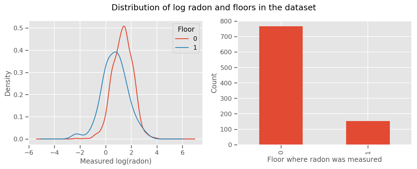
각 층 및 보편적 위해 배운 무게있다 intercept 용어. 0층과 1층의 라돈 측정값을 보면 다음과 같이 시작하는 것이 좋습니다.

fig, (ax1, ax2) = plt.subplots(ncols=2, figsize=(12, 4))
df.groupby('floor')['log_radon'].plot(kind='density', ax=ax1);
ax1.set_xlabel('Measured log(radon)')
ax1.legend(title='Floor')

df['floor'].value_counts().plot(kind='bar', ax=ax2)
ax2.set_xlabel('Floor where radon was measured')
ax2.set_ylabel('Count')
fig.suptitle("Distribution of log radon and floors in the dataset");

지리학에 대한 것을 포함하여 모델을 조금 더 정교하게 만드는 것은 아마도 훨씬 더 나을 것입니다. 라돈은 땅에 존재할 수 있는 우라늄 붕괴 사슬의 일부이므로 지리학을 설명하는 것이 핵심인 것 같습니다.

\[ \mathbb{E}[\log(\text{radon}_j)] = c + \text{floor_effect}_j + \text{county_effect}_j \]

다시, 의사 코드에서 우리는

def estimate_log_radon(floor, county):
    return intercept + floor_effect[floor] + county_effect[county]

카운티별 가중치를 제외하고는 이전과 동일합니다.

충분히 큰 훈련 세트가 주어지면 이것은 합리적인 모델입니다. 그러나 미네소타의 데이터를 고려할 때 측정 수가 적은 많은 카운티가 있음을 알 수 있습니다. 예를 들어, 85개 카운티 중 39개 카운티의 관측치가 5개 미만입니다.

이것은 카운티당 관찰 수가 증가함에 따라 위의 모델에 수렴하는 방식으로 모든 관찰 간에 통계적 강점을 공유하도록 동기를 부여합니다.

fig, ax = plt.subplots(figsize=(22, 5));
county_freq = df['county'].value_counts()
county_freq.plot(kind='bar', ax=ax)
ax.set_xlabel('County')
ax.set_ylabel('Number of readings');

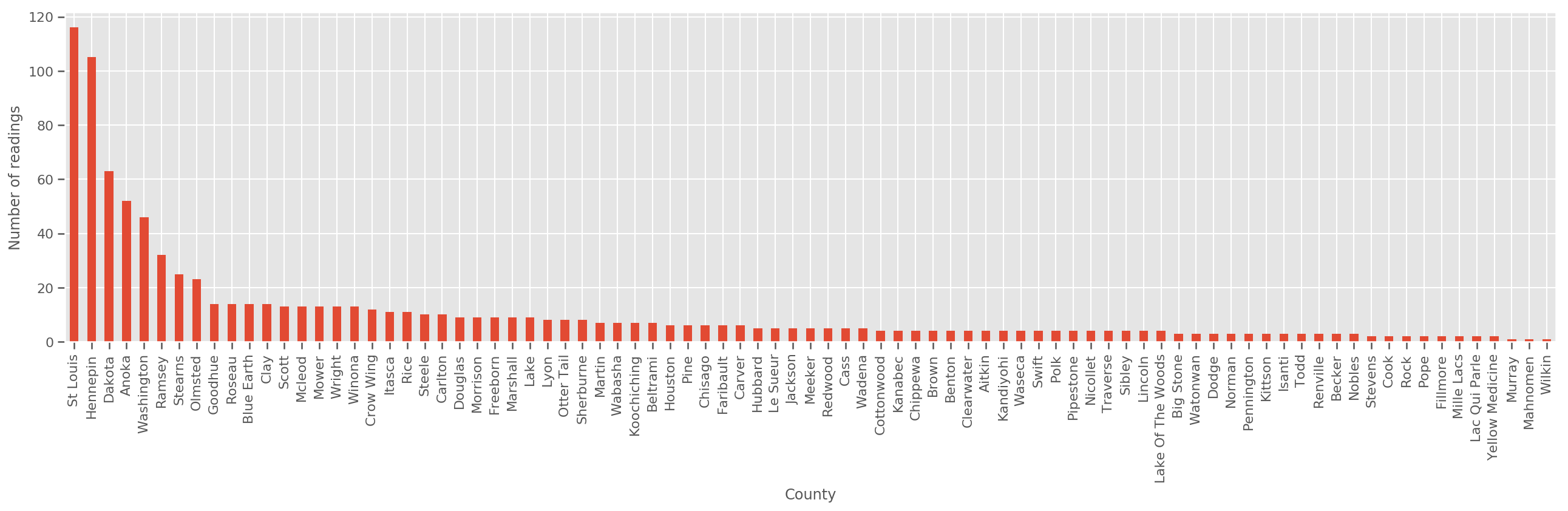
우리가이 모델을 맞는 경우, county_effect 벡터 가능성이 아마도 overfitting와 가난한 일반화로 이어지는 몇 훈련 샘플을했다 카운티의 결과를 기억 끝날 것입니다.

GLMM은 위의 두 GLM에 행복한 중간을 제공합니다. 우리는 적합을 고려할 수 있습니다

\[ \log(\text{radon}_j) \sim c + \text{floor_effect}_j + \mathcal{N}(\text{county_effect}_j, \text{county_scale}) \]

이 모델은 처음과 동일하지만, 우리는 정규 분포로 우리의 가능성을 고정해야하고, (하나의) 변수를 통해 모든 군에서 분산을 공유 할 county_scale . 의사 코드에서,

def estimate_log_radon(floor, county):
    county_mean = county_effect[county]
    random_effect = np.random.normal() * county_scale + county_mean
    return intercept + floor_effect[floor] + random_effect

우리는 이상 공동 분포를 추론 할 county_scale , county_mean 및 random_effect 우리의 관측 데이터를 사용합니다. 글로벌 county_scale 많은 관찰과 함께 그 몇 관측과 군의 분산에 타격을 제공 : 우리가 군에 걸쳐 통계 강도를 공유 할 수 있습니다. 또한 더 많은 데이터를 수집함에 따라 이 모델은 통합 척도 변수가 없는 모델로 수렴됩니다. 이 데이터 세트를 사용하더라도 두 모델 중 가장 많이 관찰된 카운티에 대해 유사한 결론에 도달할 것입니다.

실험

이제 TensorFlow에서 변형 추론을 사용하여 위의 GLMM을 맞추려고 합니다. 먼저 데이터를 기능과 레이블로 분할합니다.

features = df[['county_code', 'floor']].astype(int)
labels = df[['log_radon']].astype(np.float32).values.flatten()

모델 지정

def make_joint_distribution_coroutine(floor, county, n_counties, n_floors):

  def model():
    county_scale = yield tfd.HalfNormal(scale=1., name='scale_prior')
    intercept = yield tfd.Normal(loc=0., scale=1., name='intercept')
    floor_weight = yield tfd.Normal(loc=0., scale=1., name='floor_weight')
    county_prior = yield tfd.Normal(loc=tf.zeros(n_counties),
                                    scale=county_scale,
                                    name='county_prior')
    random_effect = tf.gather(county_prior, county, axis=-1)

    fixed_effect = intercept + floor_weight * floor
    linear_response = fixed_effect + random_effect
    yield tfd.Normal(loc=linear_response, scale=1., name='likelihood')
  return tfd.JointDistributionCoroutineAutoBatched(model)

joint = make_joint_distribution_coroutine(
    features.floor.values, features.county_code.values, df.county.nunique(),
    df.floor.nunique())

# Define a closure over the joint distribution 
# to condition on the observed labels.
def target_log_prob_fn(*args):
  return joint.log_prob(*args, likelihood=labels)

대리 사후 지정

우리는 지금 함께 대리 가족 넣어 \(q_{\lambda}\)매개 변수, \(\lambda\) 학습 가능한됩니다. 이 경우, 가족 독립 변수 정규 분포, 각 파라미터에 대해 하나, 및 \(\lambda = \{(\mu_j, \sigma_j)\}\), \(j\) 인덱스 파라미터 네.

이 방법은 우리가 대리 가족의 용도에 맞게 사용 tf.Variables . 우리는 또한 사용 tfp.util.TransformedVariable 함께 Softplus 양성하기 위해 (학습 가능한) 규모의 매개 변수를 제한 할 수 있습니다. 또한, 우리는 적용 Softplus 전체에 scale_prior 긍정적 인 매개 변수입니다.

최적화를 돕기 위해 약간의 지터를 사용하여 이러한 학습 가능한 변수를 초기화합니다.

# Initialize locations and scales randomly with `tf.Variable`s and 
# `tfp.util.TransformedVariable`s.
_init_loc = lambda shape=(): tf.Variable(
    tf.random.uniform(shape, minval=-2., maxval=2.))
_init_scale = lambda shape=(): tfp.util.TransformedVariable(
    initial_value=tf.random.uniform(shape, minval=0.01, maxval=1.),
    bijector=tfb.Softplus())
n_counties = df.county.nunique()

surrogate_posterior = tfd.JointDistributionSequentialAutoBatched([
  tfb.Softplus()(tfd.Normal(_init_loc(), _init_scale())),           # scale_prior
  tfd.Normal(_init_loc(), _init_scale()),                           # intercept
  tfd.Normal(_init_loc(), _init_scale()),                           # floor_weight
  tfd.Normal(_init_loc([n_counties]), _init_scale([n_counties]))])  # county_prior

참고이 전지로 대체 될 수 있음을 tfp.experimental.vi.build_factored_surrogate_posterior 같이 :

surrogate_posterior = tfp.experimental.vi.build_factored_surrogate_posterior(
  event_shape=joint.event_shape_tensor()[:-1],
  constraining_bijectors=[tfb.Softplus(), None, None, None])

결과

우리의 목표는 다루기 쉬운 모수화된 분포군을 정의한 다음 목표 분포에 가까운 다루기 쉬운 분포를 갖도록 모수를 선택하는 것임을 기억하십시오.

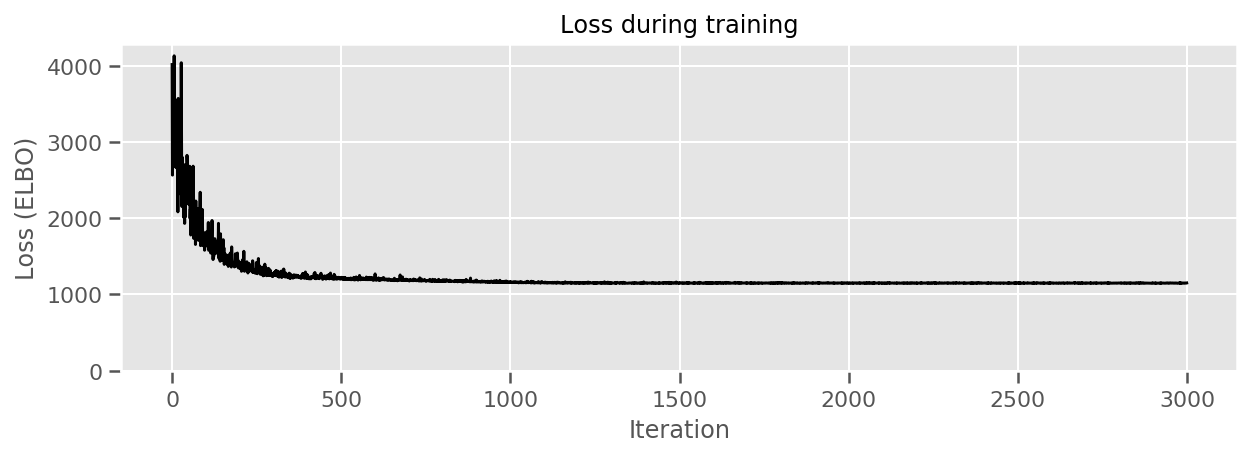
우리는 위의 대리 분포를 구축하고 사용할 수 있습니다 tfp.vi.fit_surrogate_posterior 부정적인의 ELBO을 최소화 대리 모델의 매개 변수 (사이의 쿨백 - Liebler 발산을 최소화하는 대응 될를 찾기 위해 최적화 및 단계의 주어진 숫자를 받아들이을, 대리 및 대상 분포).

반환 값은 각각의 단계에서의 부정적 ELBO이며, 분포의 surrogate_posterior 파라미터를 최적화 발견하여 업데이트 된 것이다.

optimizer = tf.optimizers.Adam(learning_rate=1e-2)

losses = tfp.vi.fit_surrogate_posterior(
    target_log_prob_fn, 
    surrogate_posterior,
    optimizer=optimizer,
    num_steps=3000, 
    seed=42,
    sample_size=2)

(scale_prior_, 
 intercept_, 
 floor_weight_, 
 county_weights_), _ = surrogate_posterior.sample_distributions()

print('        intercept (mean): ', intercept_.mean())
print('     floor_weight (mean): ', floor_weight_.mean())
print(' scale_prior (approx. mean): ', tf.reduce_mean(scale_prior_.sample(10000)))

intercept (mean):  tf.Tensor(1.4352839, shape=(), dtype=float32)
     floor_weight (mean):  tf.Tensor(-0.6701997, shape=(), dtype=float32)
 scale_prior (approx. mean):  tf.Tensor(0.28682157, shape=(), dtype=float32)

fig, ax = plt.subplots(figsize=(10, 3))
ax.plot(losses, 'k-')
ax.set(xlabel="Iteration",
       ylabel="Loss (ELBO)",
       title="Loss during training",
       ylim=0);

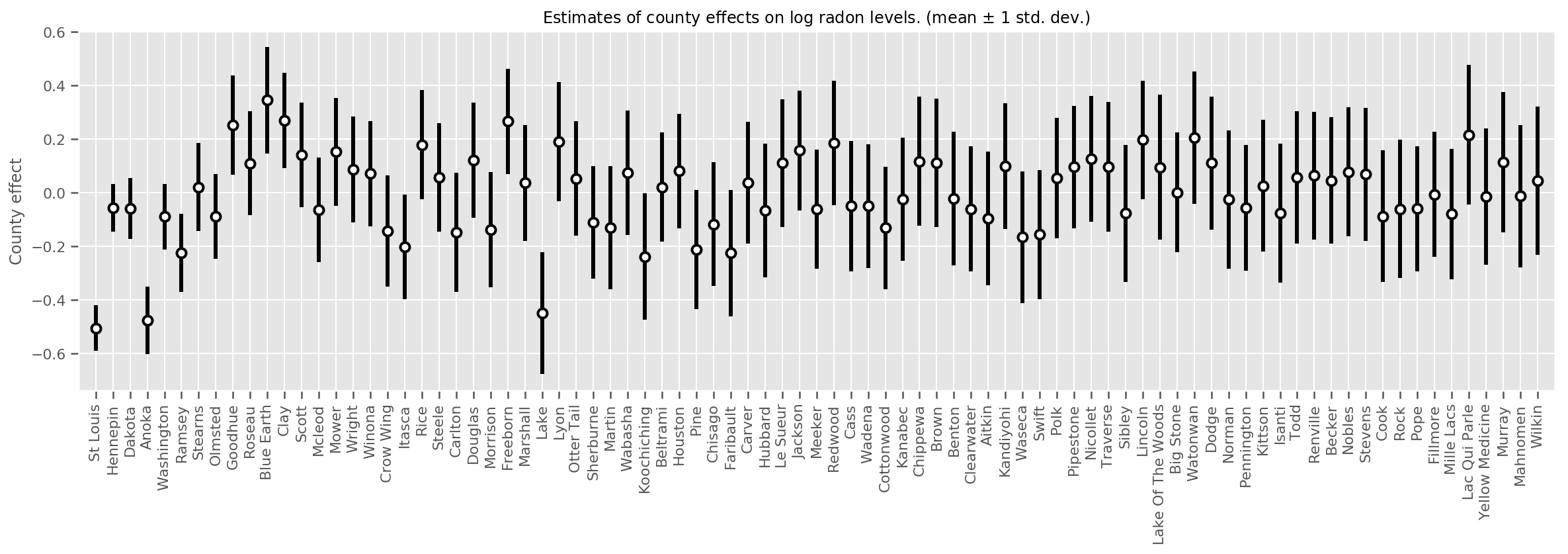
추정된 평균 카운티 효과와 해당 평균의 불확실성을 표시할 수 있습니다. 우리는 이것을 관측치의 수에 따라 정렬했으며, 가장 큰 것은 왼쪽에 있습니다. 관측치가 많은 카운티의 경우 불확실성이 작지만 관측치가 한 개 또는 두 개뿐인 카운티의 경우 불확실성이 더 큽니다.

county_counts = (df.groupby(by=['county', 'county_code'], observed=True)
                   .agg('size')
                   .sort_values(ascending=False)
                   .reset_index(name='count'))

means = county_weights_.mean()
stds = county_weights_.stddev()

fig, ax = plt.subplots(figsize=(20, 5))

for idx, row in county_counts.iterrows():
  mid = means[row.county_code]
  std = stds[row.county_code]
  ax.vlines(idx, mid - std, mid + std, linewidth=3)
  ax.plot(idx, means[row.county_code], 'ko', mfc='w', mew=2, ms=7)

ax.set(
    xticks=np.arange(len(county_counts)),
    xlim=(-1, len(county_counts)),
    ylabel="County effect",
    title=r"Estimates of county effects on log radon levels. (mean $\pm$ 1 std. dev.)",
)
ax.set_xticklabels(county_counts.county, rotation=90);

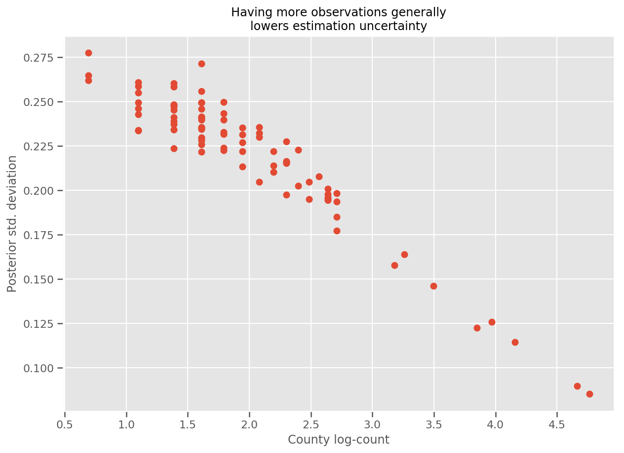
실제로 우리는 추정된 표준 편차에 대한 관측치의 로그 수를 도표화하여 이를 보다 직접적으로 볼 수 있으며 관계가 대략 선형임을 알 수 있습니다.

fig, ax = plt.subplots(figsize=(10, 7))
ax.plot(np.log1p(county_counts['count']), stds.numpy()[county_counts.county_code], 'o')
ax.set(
    ylabel='Posterior std. deviation',
    xlabel='County log-count',
    title='Having more observations generally\nlowers estimation uncertainty'
);

에 비교 lme4 R에

%%shell
exit  # Trick to make this block not execute.

radon = read.csv('srrs2.dat', header = TRUE)
radon = radon[radon$state=='MN',]
radon$radon = ifelse(radon$activity==0., 0.1, radon$activity)
radon$log_radon = log(radon$radon)

# install.packages('lme4')
library(lme4)
fit <- lmer(log_radon ~ 1 + floor + (1 | county), data=radon)
fit

# Linear mixed model fit by REML ['lmerMod']
# Formula: log_radon ~ 1 + floor + (1 | county)
#    Data: radon
# REML criterion at convergence: 2171.305
# Random effects:
#  Groups   Name        Std.Dev.
#  county   (Intercept) 0.3282
#  Residual             0.7556
# Number of obs: 919, groups:  county, 85
# Fixed Effects:
# (Intercept)        floor
#       1.462       -0.693

<IPython.core.display.Javascript at 0x7f90b888e9b0>
<IPython.core.display.Javascript at 0x7f90b888e780>
<IPython.core.display.Javascript at 0x7f90b888e780>
<IPython.core.display.Javascript at 0x7f90bce1dfd0>
<IPython.core.display.Javascript at 0x7f90b888e780>
<IPython.core.display.Javascript at 0x7f90b888e780>
<IPython.core.display.Javascript at 0x7f90b888e780>
<IPython.core.display.Javascript at 0x7f90b888e780>

다음 표에는 결과가 요약되어 있습니다.

print(pd.DataFrame(data=dict(intercept=[1.462, tf.reduce_mean(intercept_.mean()).numpy()],
                             floor=[-0.693, tf.reduce_mean(floor_weight_.mean()).numpy()],
                             scale=[0.3282, tf.reduce_mean(scale_prior_.sample(10000)).numpy()]),
                   index=['lme4', 'vi']))

intercept   floor     scale
lme4   1.462000 -0.6930  0.328200
vi     1.435284 -0.6702  0.287251

이 표는 VI 결과는 ~에서의 10 %임을 나타냅니다 lme4 의. 이것은 다음과 같은 이유로 다소 놀랍습니다.

• lme4 기반으로 라플라스 방법 (하지 VI)
• 이 colab에서 실제로 수렴하려는 노력은 없었습니다.
• 초매개변수를 조정하기 위해 최소한의 노력을 기울였습니다.
• 데이터(예: 중앙 피처 등)를 정규화하거나 사전 처리하는 노력을 기울이지 않았습니다.

결론

이 colab에서 우리는 일반화 선형 혼합 효과 모델을 설명하고 TensorFlow Probability를 사용하여 변형 추론을 사용하여 피팅하는 방법을 보여주었습니다. 장난감 문제에는 수백 개의 훈련 샘플이 있었지만 여기에 사용된 기술은 대규모로 필요한 것과 동일합니다.