| | |  Voir la source sur GitHub Voir la source sur GitHub | |
Dans cet exemple, nous montrons comment ajuster des modèles de régression à l'aide des "couches probabilistes" de TFP.
Dépendances et prérequis
Importer
from pprint import pprint
import matplotlib.pyplot as plt
import numpy as np
import seaborn as sns

import tensorflow.compat.v2 as tf
tf.enable_v2_behavior()

import tensorflow_probability as tfp

sns.reset_defaults()
#sns.set_style('whitegrid')
#sns.set_context('talk')
sns.set_context(context='talk',font_scale=0.7)

%matplotlib inline

tfd = tfp.distributions
Faites les choses rapidement !
Avant de plonger, assurons-nous que nous utilisons un GPU pour cette démo.
Pour ce faire, sélectionnez "Runtime" -> "Modifier le type d'exécution" -> "Accélérateur matériel" -> "GPU".
L'extrait suivant vérifiera que nous avons accès à un GPU.
if tf.test.gpu_device_name() != '/device:GPU:0':
  print('WARNING: GPU device not found.')
else:
  print('SUCCESS: Found GPU: {}'.format(tf.test.gpu_device_name()))
WARNING: GPU device not found.
Motivation
Ne serait-il pas formidable si nous pouvions utiliser TFP pour spécifier un modèle probabiliste, puis simplement minimiser la log-vraisemblance négative, c'est-à-dire,
negloglik = lambda y, rv_y: -rv_y.log_prob(y)
Eh bien, non seulement c'est possible, mais ce colab montre comment ! (Dans le contexte de problèmes de régression linéaire.)
Synthétiser l'ensemble de données.
w0 = 0.125
b0 = 5.
x_range = [-20, 60]

def load_dataset(n=150, n_tst=150):
  np.random.seed(43)
  def s(x):
    g = (x - x_range[0]) / (x_range[1] - x_range[0])
    return 3 * (0.25 + g**2.)
  x = (x_range[1] - x_range[0]) * np.random.rand(n) + x_range[0]
  eps = np.random.randn(n) * s(x)
  y = (w0 * x * (1. + np.sin(x)) + b0) + eps
  x = x[..., np.newaxis]
  x_tst = np.linspace(*x_range, num=n_tst).astype(np.float32)
  x_tst = x_tst[..., np.newaxis]
  return y, x, x_tst

y, x, x_tst = load_dataset()
Cas 1 : aucune incertitude
# Build model.
model = tf.keras.Sequential([
  tf.keras.layers.Dense(1),
  tfp.layers.DistributionLambda(lambda t: tfd.Normal(loc=t, scale=1)),
])

# Do inference.
model.compile(optimizer=tf.optimizers.Adam(learning_rate=0.01), loss=negloglik)
model.fit(x, y, epochs=1000, verbose=False);

# Profit.
[print(np.squeeze(w.numpy())) for w in model.weights];
yhat = model(x_tst)
assert isinstance(yhat, tfd.Distribution)
0.13032457
5.13029
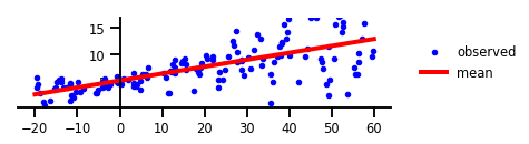
Figure 1 : Aucune incertitude.
w = np.squeeze(model.layers[-2].kernel.numpy())
b = np.squeeze(model.layers[-2].bias.numpy())

plt.figure(figsize=[6, 1.5])  # inches
#plt.figure(figsize=[8, 5])  # inches
plt.plot(x, y, 'b.', label='observed');
plt.plot(x_tst, yhat.mean(),'r', label='mean', linewidth=4);
plt.ylim(-0.,17);
plt.yticks(np.linspace(0, 15, 4)[1:]);
plt.xticks(np.linspace(*x_range, num=9));

ax=plt.gca();
ax.xaxis.set_ticks_position('bottom')
ax.yaxis.set_ticks_position('left')
ax.spines['left'].set_position(('data', 0))
ax.spines['top'].set_visible(False)
ax.spines['right'].set_visible(False)
#ax.spines['left'].set_smart_bounds(True)
#ax.spines['bottom'].set_smart_bounds(True)
plt.legend(loc='center left', fancybox=True, framealpha=0., bbox_to_anchor=(1.05, 0.5))

plt.savefig('/tmp/fig1.png', bbox_inches='tight', dpi=300)
Cas 2 : Incertitude aléatoire
# Build model.
model = tf.keras.Sequential([
  tf.keras.layers.Dense(1 + 1),
  tfp.layers.DistributionLambda(
      lambda t: tfd.Normal(loc=t[..., :1],
                           scale=1e-3 + tf.math.softplus(0.05 * t[...,1:]))),
])

# Do inference.
model.compile(optimizer=tf.optimizers.Adam(learning_rate=0.01), loss=negloglik)
model.fit(x, y, epochs=1000, verbose=False);

# Profit.
[print(np.squeeze(w.numpy())) for w in model.weights];
yhat = model(x_tst)
assert isinstance(yhat, tfd.Distribution)
[0.14738432 0.1815331 ]
[4.4812164 1.2219843]
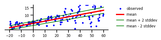
Figure 2 : Incertitude aléatoire
plt.figure(figsize=[6, 1.5])  # inches
plt.plot(x, y, 'b.', label='observed');

m = yhat.mean()
s = yhat.stddev()

plt.plot(x_tst, m, 'r', linewidth=4, label='mean');
plt.plot(x_tst, m + 2 * s, 'g', linewidth=2, label=r'mean + 2 stddev');
plt.plot(x_tst, m - 2 * s, 'g', linewidth=2, label=r'mean - 2 stddev');

plt.ylim(-0.,17);
plt.yticks(np.linspace(0, 15, 4)[1:]);
plt.xticks(np.linspace(*x_range, num=9));

ax=plt.gca();
ax.xaxis.set_ticks_position('bottom')
ax.yaxis.set_ticks_position('left')
ax.spines['left'].set_position(('data', 0))
ax.spines['top'].set_visible(False)
ax.spines['right'].set_visible(False)
#ax.spines['left'].set_smart_bounds(True)
#ax.spines['bottom'].set_smart_bounds(True)
plt.legend(loc='center left', fancybox=True, framealpha=0., bbox_to_anchor=(1.05, 0.5))

plt.savefig('/tmp/fig2.png', bbox_inches='tight', dpi=300)
Cas 3 : Incertitude épistémique
# Specify the surrogate posterior over `keras.layers.Dense` `kernel` and `bias`.
def posterior_mean_field(kernel_size, bias_size=0, dtype=None):
  n = kernel_size + bias_size
  c = np.log(np.expm1(1.))
  return tf.keras.Sequential([
      tfp.layers.VariableLayer(2 * n, dtype=dtype),
      tfp.layers.DistributionLambda(lambda t: tfd.Independent(
          tfd.Normal(loc=t[..., :n],
                     scale=1e-5 + tf.nn.softplus(c + t[..., n:])),
          reinterpreted_batch_ndims=1)),
  ])
# Specify the prior over `keras.layers.Dense` `kernel` and `bias`.
def prior_trainable(kernel_size, bias_size=0, dtype=None):
  n = kernel_size + bias_size
  return tf.keras.Sequential([
      tfp.layers.VariableLayer(n, dtype=dtype),
      tfp.layers.DistributionLambda(lambda t: tfd.Independent(
          tfd.Normal(loc=t, scale=1),
          reinterpreted_batch_ndims=1)),
  ])
# Build model.
model = tf.keras.Sequential([
  tfp.layers.DenseVariational(1, posterior_mean_field, prior_trainable, kl_weight=1/x.shape[0]),
  tfp.layers.DistributionLambda(lambda t: tfd.Normal(loc=t, scale=1)),
])

# Do inference.
model.compile(optimizer=tf.optimizers.Adam(learning_rate=0.01), loss=negloglik)
model.fit(x, y, epochs=1000, verbose=False);

# Profit.
[print(np.squeeze(w.numpy())) for w in model.weights];
yhat = model(x_tst)
assert isinstance(yhat, tfd.Distribution)
[ 0.1387333  5.125723  -4.112224  -2.2171402]
[0.12476114 5.147452  ]
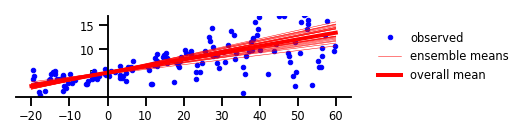
Figure 3 : Incertitude épistémique
plt.figure(figsize=[6, 1.5])  # inches
plt.clf();
plt.plot(x, y, 'b.', label='observed');

yhats = [model(x_tst) for _ in range(100)]
avgm = np.zeros_like(x_tst[..., 0])
for i, yhat in enumerate(yhats):
  m = np.squeeze(yhat.mean())
  s = np.squeeze(yhat.stddev())
  if i < 25:
    plt.plot(x_tst, m, 'r', label='ensemble means' if i == 0 else None, linewidth=0.5)
  avgm += m
plt.plot(x_tst, avgm/len(yhats), 'r', label='overall mean', linewidth=4)

plt.ylim(-0.,17);
plt.yticks(np.linspace(0, 15, 4)[1:]);
plt.xticks(np.linspace(*x_range, num=9));

ax=plt.gca();
ax.xaxis.set_ticks_position('bottom')
ax.yaxis.set_ticks_position('left')
ax.spines['left'].set_position(('data', 0))
ax.spines['top'].set_visible(False)
ax.spines['right'].set_visible(False)
#ax.spines['left'].set_smart_bounds(True)
#ax.spines['bottom'].set_smart_bounds(True)
plt.legend(loc='center left', fancybox=True, framealpha=0., bbox_to_anchor=(1.05, 0.5))

plt.savefig('/tmp/fig3.png', bbox_inches='tight', dpi=300)
Cas 4 : Incertitude aléatoire et épistémique
# Build model.
model = tf.keras.Sequential([
  tfp.layers.DenseVariational(1 + 1, posterior_mean_field, prior_trainable, kl_weight=1/x.shape[0]),
  tfp.layers.DistributionLambda(
      lambda t: tfd.Normal(loc=t[..., :1],
                           scale=1e-3 + tf.math.softplus(0.01 * t[...,1:]))),
])

# Do inference.
model.compile(optimizer=tf.optimizers.Adam(learning_rate=0.01), loss=negloglik)
model.fit(x, y, epochs=1000, verbose=False);

# Profit.
[print(np.squeeze(w.numpy())) for w in model.weights];
yhat = model(x_tst)
assert isinstance(yhat, tfd.Distribution)
[ 0.12753433  2.7504077   5.160624    3.8251898  -3.4283297  -0.8961645
 -2.2378397   0.1496858 ]
[0.14511648 2.7104297  5.1248145  3.7724588 ]
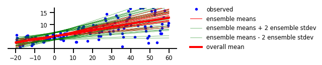
Figure 4 : Incertitude à la fois aléatoire et épistémique
plt.figure(figsize=[6, 1.5])  # inches
plt.plot(x, y, 'b.', label='observed');

yhats = [model(x_tst) for _ in range(100)]
avgm = np.zeros_like(x_tst[..., 0])
for i, yhat in enumerate(yhats):
  m = np.squeeze(yhat.mean())
  s = np.squeeze(yhat.stddev())
  if i < 15:
    plt.plot(x_tst, m, 'r', label='ensemble means' if i == 0 else None, linewidth=1.)
    plt.plot(x_tst, m + 2 * s, 'g', linewidth=0.5, label='ensemble means + 2 ensemble stdev' if i == 0 else None);
    plt.plot(x_tst, m - 2 * s, 'g', linewidth=0.5, label='ensemble means - 2 ensemble stdev' if i == 0 else None);
  avgm += m
plt.plot(x_tst, avgm/len(yhats), 'r', label='overall mean', linewidth=4)

plt.ylim(-0.,17);
plt.yticks(np.linspace(0, 15, 4)[1:]);
plt.xticks(np.linspace(*x_range, num=9));

ax=plt.gca();
ax.xaxis.set_ticks_position('bottom')
ax.yaxis.set_ticks_position('left')
ax.spines['left'].set_position(('data', 0))
ax.spines['top'].set_visible(False)
ax.spines['right'].set_visible(False)
#ax.spines['left'].set_smart_bounds(True)
#ax.spines['bottom'].set_smart_bounds(True)
plt.legend(loc='center left', fancybox=True, framealpha=0., bbox_to_anchor=(1.05, 0.5))

plt.savefig('/tmp/fig4.png', bbox_inches='tight', dpi=300)
Cas 5 : Incertitude fonctionnelle
Noyau PSD personnalisé
class RBFKernelFn(tf.keras.layers.Layer):
  def __init__(self, **kwargs):
    super(RBFKernelFn, self).__init__(**kwargs)
    dtype = kwargs.get('dtype', None)

    self._amplitude = self.add_variable(
            initializer=tf.constant_initializer(0),
            dtype=dtype,
            name='amplitude')

    self._length_scale = self.add_variable(
            initializer=tf.constant_initializer(0),
            dtype=dtype,
            name='length_scale')

  def call(self, x):
    # Never called -- this is just a layer so it can hold variables
    # in a way Keras understands.
    return x

  @property
  def kernel(self):
    return tfp.math.psd_kernels.ExponentiatedQuadratic(
      amplitude=tf.nn.softplus(0.1 * self._amplitude),
      length_scale=tf.nn.softplus(5. * self._length_scale)
    )
# For numeric stability, set the default floating-point dtype to float64
tf.keras.backend.set_floatx('float64')

# Build model.
num_inducing_points = 40
model = tf.keras.Sequential([
    tf.keras.layers.InputLayer(input_shape=[1]),
    tf.keras.layers.Dense(1, kernel_initializer='ones', use_bias=False),
    tfp.layers.VariationalGaussianProcess(
        num_inducing_points=num_inducing_points,
        kernel_provider=RBFKernelFn(),
        event_shape=[1],
        inducing_index_points_initializer=tf.constant_initializer(
            np.linspace(*x_range, num=num_inducing_points,
                        dtype=x.dtype)[..., np.newaxis]),
        unconstrained_observation_noise_variance_initializer=(
            tf.constant_initializer(np.array(0.54).astype(x.dtype))),
    ),
])

# Do inference.
batch_size = 32
loss = lambda y, rv_y: rv_y.variational_loss(
    y, kl_weight=np.array(batch_size, x.dtype) / x.shape[0])
model.compile(optimizer=tf.optimizers.Adam(learning_rate=0.01), loss=loss)
model.fit(x, y, batch_size=batch_size, epochs=1000, verbose=False)

# Profit.
yhat = model(x_tst)
assert isinstance(yhat, tfd.Distribution)
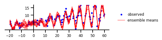
Figure 5 : Incertitude fonctionnelle
y, x, _ = load_dataset()

plt.figure(figsize=[6, 1.5])  # inches
plt.plot(x, y, 'b.', label='observed');

num_samples = 7
for i in range(num_samples):
  sample_ = yhat.sample().numpy()
  plt.plot(x_tst,
           sample_[..., 0].T,
           'r',
           linewidth=0.9,
           label='ensemble means' if i == 0 else None);

plt.ylim(-0.,17);
plt.yticks(np.linspace(0, 15, 4)[1:]);
plt.xticks(np.linspace(*x_range, num=9));

ax=plt.gca();
ax.xaxis.set_ticks_position('bottom')
ax.yaxis.set_ticks_position('left')
ax.spines['left'].set_position(('data', 0))
ax.spines['top'].set_visible(False)
ax.spines['right'].set_visible(False)
#ax.spines['left'].set_smart_bounds(True)
#ax.spines['bottom'].set_smart_bounds(True)
plt.legend(loc='center left', fancybox=True, framealpha=0., bbox_to_anchor=(1.05, 0.5))

plt.savefig('/tmp/fig5.png', bbox_inches='tight', dpi=300)