
| |
|
 在 Github 上查看源代码 在 Github 上查看源代码 |
|
在此笔记本中,我们将探索 TensorFlow Distributions(简称为 TFD)。此笔记本的目标是用通俗易懂的方式让您了解学习曲线,包括了解 TFD 对张量形状的处理。此笔记本尝试先列举示例,而不是介绍抽象的概念。我们首先介绍执行操作时公认的简单方式,而将最基本的抽象概念留到最后。如果您更偏爱较抽象的参考教程,请参阅了解 TensorFlow Distributions 形状。如果对本文介绍的内容有任何疑问,请随时联系(或加入)TensorFlow Probability 邮寄名单。我们非常乐意为您提供帮助。
首先,我们需要导入相应的库。我们的整个库为 tensorflow_probability。按照惯例,我们通常将该分布库称为 tfd。
Tensorflow Eager 是 TensorFlow 的命令式执行环境。在 TensorFlow Eager 中,每个 TF 运算都会立即得到计算并生成结果。这与 TensorFlow 的标准“计算图”模式形成对比,在“计算图”模式下,TF 运算会将节点添加到稍后执行的计算图中。整个笔记本使用 TF Eager 编写,但是本文介绍的任何概念都与其无关,并且 TFP 可以在计算图模式下使用。
import collections

import tensorflow as tf
import tensorflow_probability as tfp
tfd = tfp.distributions

try:
  tf.compat.v1.enable_eager_execution()
except ValueError:
  pass

import matplotlib.pyplot as plt
基本的一元分布
我们立即创建一个正态分布:
n = tfd.Normal(loc=0., scale=1.)
n
<tfp.distributions.Normal 'Normal' batch_shape=[] event_shape=[] dtype=float32>
我们可以通过它绘制一个样本:
n.sample()
<tf.Tensor: shape=(), dtype=float32, numpy=0.25322816>
我们可以绘制多个样本:
n.sample(3)
<tf.Tensor: shape=(3,), dtype=float32, numpy=array([-1.4658079, -0.5653636, 0.9314412], dtype=float32)>
我们可以计算一个对数概率:
n.log_prob(0.)
<tf.Tensor: shape=(), dtype=float32, numpy=-0.9189385>
我们可以计算多个对数概率:
n.log_prob([0., 2., 4.])
<tf.Tensor: shape=(3,), dtype=float32, numpy=array([-0.9189385, -2.9189386, -8.918939 ], dtype=float32)>
存在各种各样的分布。我们试一试伯努利分布:
b = tfd.Bernoulli(probs=0.7)
b
<tfp.distributions.Bernoulli 'Bernoulli' batch_shape=[] event_shape=[] dtype=int32>
b.sample()
<tf.Tensor: shape=(), dtype=int32, numpy=1>
b.sample(8)
<tf.Tensor: shape=(8,), dtype=int32, numpy=array([1, 0, 0, 0, 1, 0, 1, 0], dtype=int32)>
b.log_prob(1)
<tf.Tensor: shape=(), dtype=float32, numpy=-0.35667497>
b.log_prob([1, 0, 1, 0])
<tf.Tensor: shape=(4,), dtype=float32, numpy=array([-0.35667497, -1.2039728 , -0.35667497, -1.2039728 ], dtype=float32)>
多元分布
我们使用对角协方差创建一个多元正态分布:
nd = tfd.MultivariateNormalDiag(loc=[0., 10.], scale_diag=[1., 4.])
nd
<tfp.distributions.MultivariateNormalDiag 'MultivariateNormalDiag' batch_shape=[] event_shape=[2] dtype=float32>
将此分布与我们之前创建的一元正态分布进行比较,看看有什么不同?
tfd.Normal(loc=0., scale=1.)
<tfp.distributions.Normal 'Normal' batch_shape=[] event_shape=[] dtype=float32>
我们发现,一元正态分布的 event_shape 为 (),表明这是标量分布。多元正态分布的 event_shape 为 2,表明此分布的基本事件空间为二维空间。
抽样的工作方式与以前相同:
nd.sample()
<tf.Tensor: shape=(2,), dtype=float32, numpy=array([-1.2489667, 15.025171 ], dtype=float32)>
nd.sample(5)
<tf.Tensor: shape=(5, 2), dtype=float32, numpy=
array([[-1.5439653 ,  8.9968405 ],
       [-0.38730723, 12.448896  ],
       [-0.8697963 ,  9.330035  ],
       [-1.2541095 , 10.268944  ],
       [ 2.3475595 , 13.184147  ]], dtype=float32)>
nd.log_prob([0., 10])
<tf.Tensor: shape=(), dtype=float32, numpy=-3.2241714>
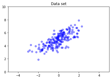
多元正态分布通常没有对角协方差。通过 TFD,可以采用多种方式创建多元正态分布,包括完全协方差规范(由协方差矩阵的 Cholesky 因子参数化),也就是我们在本文中使用的规范。
covariance_matrix = [[1., .7], [.7, 1.]]
nd = tfd.MultivariateNormalTriL(
    loc = [0., 5], scale_tril = tf.linalg.cholesky(covariance_matrix))
data = nd.sample(200)
plt.scatter(data[:, 0], data[:, 1], color='blue', alpha=0.4)
plt.axis([-5, 5, 0, 10])
plt.title("Data set")
plt.show()
多个分布
我们介绍的第一个伯努利分布表示公平地抛掷一枚硬币。我们也可以在一个 Distribution 对象中创建一批独立的伯努利分布,每个分布具有自己的参数:
b3 = tfd.Bernoulli(probs=[.3, .5, .7])
b3
<tfp.distributions.Bernoulli 'Bernoulli' batch_shape=[3] event_shape=[] dtype=int32>
重要的是弄清楚其具体含义。上述调用定义了三个独立的伯努利分布,它们恰好都在同一个 Python Distribution 对象中。这三个分布无法分别操作。请注意,batch_shape 为 (3,),表明该批次包含三个分布,event_shape 为 (),表明各个分布具有一元事件空间。
如果我们调用 sample,将得到所有这三个分布的样本:
b3.sample()
<tf.Tensor: shape=(3,), dtype=int32, numpy=array([0, 1, 1], dtype=int32)>
b3.sample(6)
<tf.Tensor: shape=(6, 3), dtype=int32, numpy=
array([[1, 0, 1],
       [0, 1, 1],
       [0, 0, 1],
       [0, 0, 1],
       [0, 0, 1],
       [0, 1, 0]], dtype=int32)>
如果调用 prob(其形状语义与 log_prob 相同;为了清楚起见,我们将 prob 与这些小的伯努利示例结合使用,但是 log_prob 通常更适合在应用中使用),我们可以向其传递一个向量,并计算抛掷每个硬币时得到该值的概率:
b3.prob([1, 1, 0])
<tf.Tensor: shape=(3,), dtype=float32, numpy=array([0.29999998, 0.5 , 0.29999998], dtype=float32)>
API 为何会包含批次形状?从语义上来讲,API 可以创建一组分布并使用 for 循环(至少在 Eager 模式下如此;在 TF 计算图模式下,需要使用 tf.while 循环)对这些分布进行迭代,从而执行相同的计算。但是,极为常见的情况是一组(可能较大的)分布采用相同的参数设置;为了能够使用硬件加速器快速进行计算,关键要素是尽可能使用向量化计算。
使用 Independent 将批次汇总到事件
在上一部分中,我们创建了单个 Distribution 对象 b3,它表示抛掷硬币三次。如果我们在向量 \(v\) 上调用 b3.prob,第 \(i\) 个条目就是抛掷第 \(i\) 枚硬币时得到的值为 \(v[i]\) 的概率。
假设我们改为对同一底层系列中的独立随机变量指定“联合”分布。这是不同的数学对象,因为在这个新分布中,向量 \(v\) 的 prob 将返回单个值,表示抛掷整组硬币时得到的值均为向量 \(v\) 的概率。
我们如何实现这个目标呢?我们使用名为 Independent 的“高阶”分布,它获取一个分布,并得到一个批次形状移动至事件形状的新分布:
b3_joint = tfd.Independent(b3, reinterpreted_batch_ndims=1)
b3_joint
<tfp.distributions.Independent 'IndependentBernoulli' batch_shape=[] event_shape=[3] dtype=int32>
将该形状与原始 b3 的形状进行比较:
b3
<tfp.distributions.Bernoulli 'Bernoulli' batch_shape=[3] event_shape=[] dtype=int32>
如前所述,我们发现 Independent 已将批次形状移动至事件形状:b3_joint 是三维事件空间 (event_shape = (3,)) 上的单一分布 (batch_shape = ())。
我们检查语义:
b3_joint.prob([1, 1, 0])
<tf.Tensor: shape=(), dtype=float32, numpy=0.044999998>
通过另一种方式也可以获得相同的结果,也就是使用 b3 计算概率,并通过乘法(或者采用更常见的做法,即使用对数概率,求和)手动简化:
tf.reduce_prod(b3.prob([1, 1, 0]))
<tf.Tensor: shape=(), dtype=float32, numpy=0.044999994>
借助 Indpendent,用户可以更明确地表示所需的概念。我们将其视为极为有用的标记,但是它并不完全必要。
以下事实较为有趣:
b3.sample和b3_joint.sample采用不同的概念实现,但输出无区别:在计算概率时,使用Independent基于批次生成的一批独立分布与单个分布之间存在差异,但在抽样时,这两种分布之间没有差别。- 可以使用标量
Normal和Independent分布轻松实现MultivariateNormalDiag(实际上不会以这种方式来实现它,但可以这么做)。
多元分布的批次
我们创建一个批次,其中包含三个完全协方差的二维多元正态分布:
covariance_matrix = [[[1., .1], [.1, 1.]],
                      [[1., .3], [.3, 1.]],
                      [[1., .5], [.5, 1.]]]
nd_batch = tfd.MultivariateNormalTriL(
    loc = [[0., 0.], [1., 1.], [2., 2.]],
    scale_tril = tf.linalg.cholesky(covariance_matrix))
nd_batch
<tfp.distributions.MultivariateNormalTriL 'MultivariateNormalTriL' batch_shape=[3] event_shape=[2] dtype=float32>
我们发现 batch_shape = (3,),因此,有三个独立的多元正态分布;event_shape = (2,),因此,每个多元正态分布均为二维分布。在本例中,单个分布没有独立的元素。
抽样如下:
nd_batch.sample(4)
<tf.Tensor: shape=(4, 3, 2), dtype=float32, numpy=
array([[[ 0.7367498 ,  2.730996  ],
        [-0.74080074, -0.36466932],
        [ 0.6516018 ,  0.9391426 ]],

       [[ 1.038303  ,  0.12231752],
        [-0.94788766, -1.204232  ],
        [ 4.059758  ,  3.035752  ]],

       [[ 0.56903946, -0.06875849],
        [-0.35127294,  0.5311631 ],
        [ 3.4635801 ,  4.565582  ]],

       [[-0.15989424, -0.25715637],
        [ 0.87479895,  0.97391707],
        [ 0.5211419 ,  2.32108   ]]], dtype=float32)>
由于 batch_shape = (3,) 并且 event_shape = (2,),我们将形状张量 (3, 2) 传递给 log_prob:
nd_batch.log_prob([[0., 0.], [1., 1.], [2., 2.]])
<tf.Tensor: shape=(3,), dtype=float32, numpy=array([-1.8328519, -1.7907217, -1.694036 ], dtype=float32)>
广播(也可以说这为何让人如此困惑?)
到目前为止,我们所执行的操作可以抽象概括为,每个分布都有一个批次形状 B 和一个事件形状 E。令 BE 作为事件形状的串联:
- 对于一元标量分布
n和b,BE = ()。 - 对于二维多元正态分布
nd,BE = (2)。 - 对于
b3和b3_joint,BE = (3)。 - 对于多元正态分布批次
ndb,BE = (3, 2)。
到目前为止,我们使用的“计算规则”如下:
- 没有参数的样本将返回形状为
BE的张量;标量为 n 的抽样将返回张量“n *BE”。 prob和log_prob使用形状为BE的张量,并返回形状为B的结果。
prob 和 log_prob 的实际“计算规则”更复杂,虽然性能和速度可能不错,但同时也增加了复杂性和挑战。实际规则(本质上)是 {nbsp}log_prob 的参数必须可以根据 BE 进行广播;输出中会预留“额外”维度。
我们来探索具体含义。对于一元正态分布 n,BE = (),因此,log_prob 应该为标量。如果我们向 log_prob 传递具有非空形状的张量,它们在输出中将显示为批次维度:
n = tfd.Normal(loc=0., scale=1.)
n
<tfp.distributions.Normal 'Normal' batch_shape=[] event_shape=[] dtype=float32>
n.log_prob(0.)
<tf.Tensor: shape=(), dtype=float32, numpy=-0.9189385>
n.log_prob([0.])
<tf.Tensor: shape=(1,), dtype=float32, numpy=array([-0.9189385], dtype=float32)>
n.log_prob([[0., 1.], [-1., 2.]])
<tf.Tensor: shape=(2, 2), dtype=float32, numpy=
array([[-0.9189385, -1.4189385],
       [-1.4189385, -2.9189386]], dtype=float32)>
我们转到二维多元正态分布 nd(为了便于阐述,对参数进行了更改):
nd = tfd.MultivariateNormalDiag(loc=[0., 1.], scale_diag=[1., 1.])
nd
<tfp.distributions.MultivariateNormalDiag 'MultivariateNormalDiag' batch_shape=[] event_shape=[2] dtype=float32>
log_prob“应该”使用形状为 (2,) 的参数,但它将接受根据此形状广播的任何参数:
nd.log_prob([0., 0.])
<tf.Tensor: shape=(), dtype=float32, numpy=-2.337877>
不过,我们可以传入“更多”示例,并同时计算所有 log_prob:
nd.log_prob([[0., 0.],
             [1., 1.],
             [2., 2.]])
<tf.Tensor: shape=(3,), dtype=float32, numpy=array([-2.337877 , -2.337877 , -4.3378773], dtype=float32)>
说服力可能还不够强,我们可以在事件维度上广播:
nd.log_prob([0.])
<tf.Tensor: shape=(), dtype=float32, numpy=-2.337877>
nd.log_prob([[0.], [1.], [2.]])
<tf.Tensor: shape=(3,), dtype=float32, numpy=array([-2.337877 , -2.337877 , -4.3378773], dtype=float32)>
这样广播后,我们最后得到了“尽可能广播”的设计;这种用法存在一些争议,在以后的 TFP 版本中可能会被移除。
现在,我们再来看看三枚硬币的示例:
b3 = tfd.Bernoulli(probs=[.3, .5, .7])
在此,可以非常直观地使用广播来表示每一枚硬币正面朝上的概率:
b3.prob([1])
<tf.Tensor: shape=(3,), dtype=float32, numpy=array([0.29999998, 0.5 , 0.7 ], dtype=float32)>
(将其与 b3.prob([1., 1., 1.]) 进行比较,我们在前面介绍 b3 时使用过后者。)
现在,假设我们想知道,对于每一枚硬币,硬币正面朝上的概率和背面朝上的概率。我们可以尝试:
b3.log_prob([0, 1])
遗憾的是,这样会得到错误,其中包含可辨识度较低的长堆栈轨迹。对于 b3,BE = (3),因此,我们必须向 b3.prob 传递可根据 (3,) 进行广播的内容。[0, 1] 的形状为 (2),因此,它不会广播,也不会生成错误。相反,我们必须使用:
b3.prob([[0], [1]])
<tf.Tensor: shape=(2, 3), dtype=float32, numpy=
array([[0.7, 0.5, 0.3],
       [0.3, 0.5, 0.7]], dtype=float32)>
原因是 [[0], [1]] 的形状为 (2, 1),因此,它会根据形状 (3) 广播,从而生成 (2, 3) 的广播形状。
广播非常有用:在有些情况下,广播可以大幅减少所使用的内存量,并且通常可以缩短用户代码。但是,广播对程序来说是一项挑战。如果调用 log_prob 并得到错误,问题几乎总是广播失败。
延伸内容
在本教程中,我们进行了简单介绍(希望如此)。作为延伸内容,有以下几点建议:
event_shape、batch_shape和sample_shape可以是任意秩(在本教程中,它们始终为标量或秩 1)。这可以提高性能,但也会为编程带来挑战,特别是在涉及到广播时。要想深入了解形状操作,请参阅 了解 TensorFlow Distributions 形状。- TFP 包含一个强大的抽象概念
Bijectors,将该概念与TransformedDistribution结合使用,可以轻松灵活地创建新的分布,这些分布是现有分布的可逆转换。我们很快会尝试编写相关的教程,但目前可以参阅本文档。