
| |  GitHubでソースを表示 GitHubでソースを表示 | |
このチュートリアルでは、古典的なニューラルネットワークがキュービットキャリブレーションエラーを修正する方法を学習する方法を示します。ノイズの多い中間スケールクォンタム(NISQ)回路を作成、編集、呼び出すためのPythonフレームワークであるCirqを紹介し、CirqがTensorFlowQuantumとどのようにインターフェースするかを示します。
設定
pip install tensorflow==2.7.0
TensorFlowQuantumをインストールします。
pip install tensorflow-quantum
# Update package resources to account for version changes.
import importlib, pkg_resources
importlib.reload(pkg_resources)
<module 'pkg_resources' from '/tmpfs/src/tf_docs_env/lib/python3.7/site-packages/pkg_resources/__init__.py'>
次に、TensorFlowとモジュールの依存関係をインポートします。
import tensorflow as tf
import tensorflow_quantum as tfq

import cirq
import sympy
import numpy as np

# visualization tools
%matplotlib inline
import matplotlib.pyplot as plt
from cirq.contrib.svg import SVGCircuit
2022-02-04 12:27:31.677071: E tensorflow/stream_executor/cuda/cuda_driver.cc:271] failed call to cuInit: CUDA_ERROR_NO_DEVICE: no CUDA-capable device is detected
1.基本
1.1回路とパラメータ化された量子回路
TensorFlow Quantum(TFQ)を探索する前に、 Cirqの基本をいくつか見てみましょう。 Cirqは、Googleの量子コンピューティング用のPythonライブラリです。これを使用して、静的ゲートやパラメータ化されたゲートなどの回路を定義します。
CirqはSymPyシンボルを使用して自由パラメーターを表します。
a, b = sympy.symbols('a b')
次のコードは、パラメータを使用して2キュービット回路を作成します。
# Create two qubits
q0, q1 = cirq.GridQubit.rect(1, 2)

# Create a circuit on these qubits using the parameters you created above.
circuit = cirq.Circuit(
    cirq.rx(a).on(q0),
    cirq.ry(b).on(q1), cirq.CNOT(control=q0, target=q1))

SVGCircuit(circuit)
findfont: Font family ['Arial'] not found. Falling back to DejaVu Sans.

回路を評価するには、 cirq.Simulatorインターフェースを使用できます。 cirq.ParamResolverオブジェクトを渡すことにより、回路内の自由パラメーターを特定の数値に置き換えます。次のコードは、パラメータ化された回路の生の状態ベクトル出力を計算します。
# Calculate a state vector with a=0.5 and b=-0.5.
resolver = cirq.ParamResolver({a: 0.5, b: -0.5})
output_state_vector = cirq.Simulator().simulate(circuit, resolver).final_state_vector
output_state_vector
array([ 0.9387913 +0.j        , -0.23971277+0.j        ,

        0.        +0.06120872j,  0.        -0.23971277j], dtype=complex64)
状態ベクトルは、シミュレーションの外部から直接アクセスすることはできません(上記の出力の複素数に注意してください)。物理的に現実的にするには、測定値を指定する必要があります。これにより、状態ベクトルが従来のコンピューターで理解できる実数に変換されます。 Cirqは、パウリ演算子 \(\hat{X}\)、 \(\hat{Y}\)、および \(\hat{Z}\)の組み合わせを使用して測定値を指定します。例として、次のコードは、シミュレートした状態ベクトルのl10n \(\hat{Z}_0\) と \(\frac{1}{2}\hat{Z}_0 + \hat{X}_1\) placeholder5を測定します。
z0 = cirq.Z(q0)

qubit_map={q0: 0, q1: 1}

z0.expectation_from_state_vector(output_state_vector, qubit_map).real
0.8775825500488281
z0x1 = 0.5 * z0 + cirq.X(q1)

z0x1.expectation_from_state_vector(output_state_vector, qubit_map).real
-0.04063427448272705
1.2テンソルとしての量子回路
TensorFlow Quantum(TFQ)は、Cirqオブジェクトをテンソルに変換する関数であるtfq.convert_to_tensorを提供します。これにより、Cirqオブジェクトをクォンタムレイヤーとクォンタムオペレーションに送信できます。この関数は、CirqCircuitsとCirqPaulisのリストまたは配列で呼び出すことができます。
# Rank 1 tensor containing 1 circuit.
circuit_tensor = tfq.convert_to_tensor([circuit])

print(circuit_tensor.shape)
print(circuit_tensor.dtype)
(1,)
<dtype: 'string'>
プレースホルダー28
これは、Cirqオブジェクトをtf.stringテンソルとしてエンコードし、 tfq操作が必要に応じてデコードします。
# Rank 1 tensor containing 2 Pauli operators.
pauli_tensor = tfq.convert_to_tensor([z0, z0x1])
pauli_tensor.shape
TensorShape([2])
1.3バッチ回路シミュレーション
TFQは、期待値、サンプル、および状態ベクトルを計算するためのメソッドを提供します。今のところ、期待値に焦点を当てましょう。
期待値を計算するための最高レベルのインターフェースは、 tf.keras.Layerであるtfq.layers.Expectationレイヤーです。最も単純な形式では、このレイヤーは、多くのcirq.ParamResolversでパラメーター化された回路をシミュレートするのと同じです。ただし、TFQではTensorFlowセマンティクスに従ったバッチ処理が可能であり、回路は効率的なC ++コードを使用してシミュレートされます。
aパラメータとbパラメータの代わりに値のバッチを作成します。
batch_vals = np.array(np.random.uniform(0, 2 * np.pi, (5, 2)), dtype=np.float32)
Cirqのパラメーター値に対する回路実行のバッチ処理には、ループが必要です。
cirq_results = []
cirq_simulator = cirq.Simulator()

for vals in batch_vals:
    resolver = cirq.ParamResolver({a: vals[0], b: vals[1]})
    final_state_vector = cirq_simulator.simulate(circuit, resolver).final_state_vector
    cirq_results.append(
        [z0.expectation_from_state_vector(final_state_vector, {
            q0: 0,
            q1: 1
        }).real])

print('cirq batch results: \n {}'.format(np.array(cirq_results)))
cirq batch results:
 [[-0.66652703]
 [ 0.49764055]
 [ 0.67326665]
 [-0.95549959]
 [-0.81297827]]
同じ操作がTFQで簡略化されています。
tfq.layers.Expectation()(circuit,
                         symbol_names=[a, b],
                         symbol_values=batch_vals,
                         operators=z0)
<tf.Tensor: shape=(5, 1), dtype=float32, numpy=
array([[-0.666526  ],
       [ 0.49764216],
       [ 0.6732664 ],
       [-0.9554999 ],
       [-0.8129788 ]], dtype=float32)>
2.ハイブリッド量子-古典的最適化
基本を理解したので、TensorFlowQuantumを使用してハイブリッド量子-古典的ニューラルネットを構築しましょう。単一のキュービットを制御するために、古典的なニューラルネットをトレーニングします。コントロールは、 0または1状態のキュービットを正しく準備するように最適化され、シミュレートされた体系的なキャリブレーションエラーを克服します。この図は、アーキテクチャを示しています。
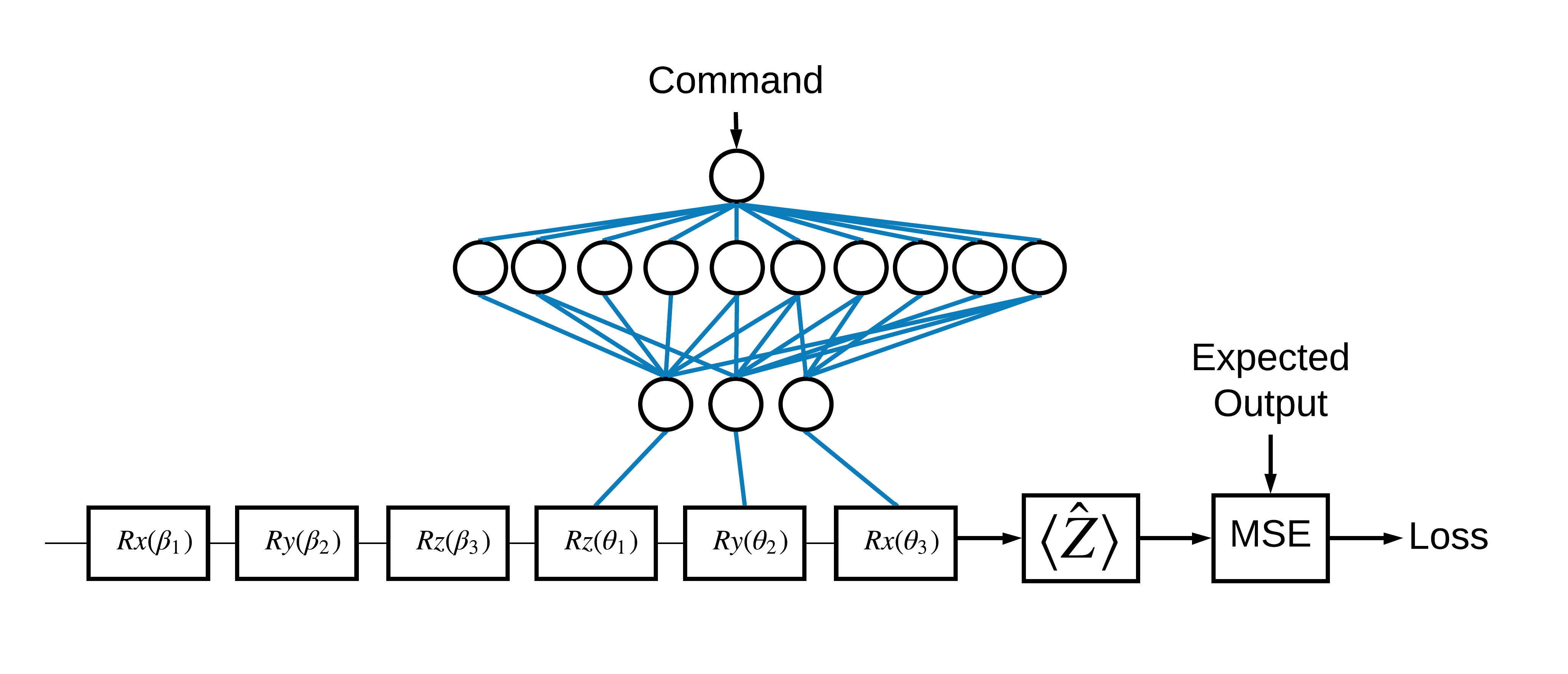
ニューラルネットワークがなくても、これは簡単に解決できる問題ですが、テーマは、TFQを使用して解決できる実際の量子制御の問題に似ています。これは、 tf.keras.Model内のtfq.layers.ControlledPQC (Parametrized Quantum Circuit)レイヤーを使用した量子古典的計算のエンドツーエンドの例を示しています。
このチュートリアルの実装では、このアーキテクチャは3つの部分に分かれています。
- 入力回路またはデータポイント回路:最初の3つの \(R\) ゲート。
- 制御回路:他の3つの \(R\) ゲート。
- コントローラー:制御回路のパラメーターを設定する古典的なニューラルネットワーク。
2.1制御回路の定義
上の図に示すように、学習可能なシングルビットローテーションを定義します。これは私たちの制御回路に対応します。
# Parameters that the classical NN will feed values into.
control_params = sympy.symbols('theta_1 theta_2 theta_3')

# Create the parameterized circuit.
qubit = cirq.GridQubit(0, 0)
model_circuit = cirq.Circuit(
    cirq.rz(control_params[0])(qubit),
    cirq.ry(control_params[1])(qubit),
    cirq.rx(control_params[2])(qubit))

SVGCircuit(model_circuit)

2.2コントローラー
次に、コントローラーネットワークを定義します。
# The classical neural network layers.
controller = tf.keras.Sequential([
    tf.keras.layers.Dense(10, activation='elu'),
    tf.keras.layers.Dense(3)
])
コマンドのバッチが与えられると、コントローラは制御された回路の制御信号のバッチを出力します。
コントローラはランダムに初期化されるため、これらの出力はまだ役に立ちません。
controller(tf.constant([[0.0],[1.0]])).numpy()
array([[0.        , 0.        , 0.        ],
       [0.5815686 , 0.21376055, 0.57181627]], dtype=float32)
2.3コントローラーを回路に接続します
tfqを使用して、コントローラーを単一のkeras.Modelとして制御回路に接続します。
このスタイルのモデル定義の詳細については、 Keras FunctionalAPIガイドを参照してください。
まず、モデルへの入力を定義します。
# This input is the simulated miscalibration that the model will learn to correct.
circuits_input = tf.keras.Input(shape=(),
                                # The circuit-tensor has dtype `tf.string`
                                dtype=tf.string,
                                name='circuits_input')

# Commands will be either `0` or `1`, specifying the state to set the qubit to.
commands_input = tf.keras.Input(shape=(1,),
                                dtype=tf.dtypes.float32,
                                name='commands_input')
次に、これらの入力に操作を適用して、計算を定義します。
dense_2 = controller(commands_input)

# TFQ layer for classically controlled circuits.
expectation_layer = tfq.layers.ControlledPQC(model_circuit,
                                             # Observe Z
                                             operators = cirq.Z(qubit))
expectation = expectation_layer([circuits_input, dense_2])
次に、この計算をtf.keras.Modelとしてパッケージ化します。
# The full Keras model is built from our layers.
model = tf.keras.Model(inputs=[circuits_input, commands_input],
                       outputs=expectation)
ネットワークアーキテクチャは、以下のモデルのプロットで示されています。このモデルプロットをアーキテクチャ図と比較して、正確さを確認します。
tf.keras.utils.plot_model(model, show_shapes=True, dpi=70)
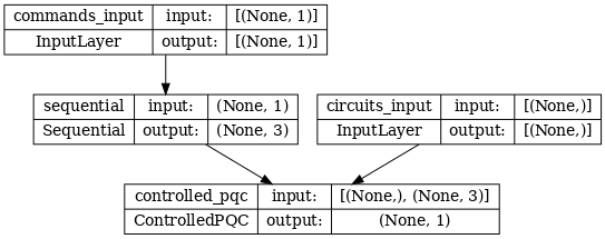
このモデルは、2つの入力を受け取ります。コントローラーのコマンドと、コントローラーが出力を修正しようとしている入力回路です。
2.4データセット
モデルは、コマンドごとに \(\hat{Z}\) の正しい正しい測定値を出力しようとします。コマンドと正しい値を以下に定義します。
# The command input values to the classical NN.
commands = np.array([[0], [1]], dtype=np.float32)

# The desired Z expectation value at output of quantum circuit.
expected_outputs = np.array([[1], [-1]], dtype=np.float32)
これは、このタスクのトレーニングデータセット全体ではありません。データセット内の各データポイントにも入力回路が必要です。
2.4入力回路の定義
以下の入力回路は、モデルが修正することを学習するランダムな誤校正を定義します。
random_rotations = np.random.uniform(0, 2 * np.pi, 3)
noisy_preparation = cirq.Circuit(
  cirq.rx(random_rotations[0])(qubit),
  cirq.ry(random_rotations[1])(qubit),
  cirq.rz(random_rotations[2])(qubit)
)
datapoint_circuits = tfq.convert_to_tensor([
  noisy_preparation
] * 2)  # Make two copied of this circuit
回路のコピーは2つあり、データポイントごとに1つです。
datapoint_circuits.shape
TensorShape([2])
2.5トレーニング
定義された入力を使用して、 tfqモデルをテスト実行できます。
model([datapoint_circuits, commands]).numpy()
array([[0.95853525],
       [0.6272128 ]], dtype=float32)
プレースホルダー49次に、標準のトレーニングプロセスを実行して、これらの値をexpected_outputsに向けて調整します。
optimizer = tf.keras.optimizers.Adam(learning_rate=0.05)
loss = tf.keras.losses.MeanSquaredError()
model.compile(optimizer=optimizer, loss=loss)
history = model.fit(x=[datapoint_circuits, commands],
                    y=expected_outputs,
                    epochs=30,
                    verbose=0)
plt.plot(history.history['loss'])
plt.title("Learning to Control a Qubit")
plt.xlabel("Iterations")
plt.ylabel("Error in Control")
plt.show()
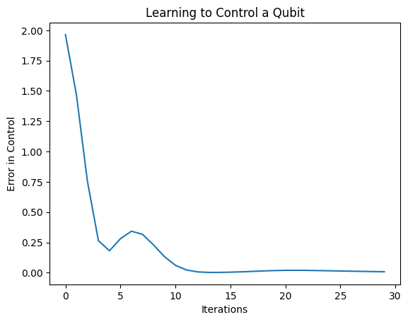
このプロットから、ニューラルネットワークが体系的な誤校正を克服することを学習したことがわかります。
2.6出力を確認する
次に、トレーニング済みモデルを使用して、キュービットキャリブレーションエラーを修正します。 Cirqの場合:
def check_error(command_values, desired_values):
  """Based on the value in `command_value` see how well you could prepare
  the full circuit to have `desired_value` when taking expectation w.r.t. Z."""
  params_to_prepare_output = controller(command_values).numpy()
  full_circuit = noisy_preparation + model_circuit

  # Test how well you can prepare a state to get expectation the expectation
  # value in `desired_values`
  for index in [0, 1]:
    state = cirq_simulator.simulate(
        full_circuit,
        {s:v for (s,v) in zip(control_params, params_to_prepare_output[index])}
    ).final_state_vector
    expt = cirq.Z(qubit).expectation_from_state_vector(state, {qubit: 0}).real
    print(f'For a desired output (expectation) of {desired_values[index]} with'
          f' noisy preparation, the controller\nnetwork found the following '
          f'values for theta: {params_to_prepare_output[index]}\nWhich gives an'
          f' actual expectation of: {expt}\n')


check_error(commands, expected_outputs)
For a desired output (expectation) of [1.] with noisy preparation, the controller
network found the following values for theta: [-0.6788422   0.3395225  -0.59394693]
Which gives an actual expectation of: 0.9171845316886902

For a desired output (expectation) of [-1.] with noisy preparation, the controller
network found the following values for theta: [-5.203663   -0.29528576  3.2887425 ]
Which gives an actual expectation of: -0.9511058330535889
トレーニング中の損失関数の値は、モデルがどれだけうまく学習しているかの大まかなアイデアを提供します。損失が小さいほど、上記のセルの期待値はdesired_valuesに近くなります。パラメータ値に関心がない場合は、 tfqを使用して上記の出力をいつでも確認できます。
model([datapoint_circuits, commands])
<tf.Tensor: shape=(2, 1), dtype=float32, numpy=
array([[ 0.91718477],
       [-0.9511056 ]], dtype=float32)>
3さまざまな演算子の固有状態を準備する方法を学ぶ
1と0に対応する \(\pm \hat{Z}\) 固有状態の選択は任意でした。 1を \(+ \hat{Z}\) \(-\hat{X}\) 状態に対応させることも簡単にできます。これを実現する1つの方法は、次の図に示すように、コマンドごとに異なる測定演算子を指定することです。

これには、 tfq.layers.Expectationを使用する必要があります。これで、入力は、回路、コマンド、および演算子の3つのオブジェクトを含むようになりました。出力は依然として期待値です。
3.1新しいモデルの定義
このタスクを実行するためのモデルを見てみましょう。
# Define inputs.
commands_input = tf.keras.layers.Input(shape=(1),
                                       dtype=tf.dtypes.float32,
                                       name='commands_input')
circuits_input = tf.keras.Input(shape=(),
                                # The circuit-tensor has dtype `tf.string`
                                dtype=tf.dtypes.string,
                                name='circuits_input')
operators_input = tf.keras.Input(shape=(1,),
                                 dtype=tf.dtypes.string,
                                 name='operators_input')
コントローラネットワークは次のとおりです。
# Define classical NN.
controller = tf.keras.Sequential([
    tf.keras.layers.Dense(10, activation='elu'),
    tf.keras.layers.Dense(3)
])
回路とコントローラーを1つのkerasに結合しますkeras.Modelを使用したtfq :
dense_2 = controller(commands_input)

# Since you aren't using a PQC or ControlledPQC you must append
# your model circuit onto the datapoint circuit tensor manually.
full_circuit = tfq.layers.AddCircuit()(circuits_input, append=model_circuit)
expectation_output = tfq.layers.Expectation()(full_circuit,
                                              symbol_names=control_params,
                                              symbol_values=dense_2,
                                              operators=operators_input)

# Contruct your Keras model.
two_axis_control_model = tf.keras.Model(
    inputs=[circuits_input, commands_input, operators_input],
    outputs=[expectation_output])
3.2データセット
ここで、 model_circuitに提供する各データポイントに対して測定する演算子も含めます。
# The operators to measure, for each command.
operator_data = tfq.convert_to_tensor([[cirq.X(qubit)], [cirq.Z(qubit)]])

# The command input values to the classical NN.
commands = np.array([[0], [1]], dtype=np.float32)

# The desired expectation value at output of quantum circuit.
expected_outputs = np.array([[1], [-1]], dtype=np.float32)
3.3トレーニング
新しい入力と出力ができたので、kerasを使用してもう一度トレーニングできます。
optimizer = tf.keras.optimizers.Adam(learning_rate=0.05)
loss = tf.keras.losses.MeanSquaredError()

two_axis_control_model.compile(optimizer=optimizer, loss=loss)

history = two_axis_control_model.fit(
    x=[datapoint_circuits, commands, operator_data],
    y=expected_outputs,
    epochs=30,
    verbose=1)
Epoch 1/30
1/1 [==============================] - 0s 320ms/step - loss: 2.4404
Epoch 2/30
1/1 [==============================] - 0s 3ms/step - loss: 1.8713
Epoch 3/30
1/1 [==============================] - 0s 3ms/step - loss: 1.1400
Epoch 4/30
1/1 [==============================] - 0s 3ms/step - loss: 0.5071
Epoch 5/30
1/1 [==============================] - 0s 3ms/step - loss: 0.1611
Epoch 6/30
1/1 [==============================] - 0s 3ms/step - loss: 0.0426
Epoch 7/30
1/1 [==============================] - 0s 3ms/step - loss: 0.0117
Epoch 8/30
1/1 [==============================] - 0s 3ms/step - loss: 0.0032
Epoch 9/30
1/1 [==============================] - 0s 2ms/step - loss: 0.0147
Epoch 10/30
1/1 [==============================] - 0s 3ms/step - loss: 0.0452
Epoch 11/30
1/1 [==============================] - 0s 3ms/step - loss: 0.0670
Epoch 12/30
1/1 [==============================] - 0s 3ms/step - loss: 0.0648
Epoch 13/30
1/1 [==============================] - 0s 3ms/step - loss: 0.0471
Epoch 14/30
1/1 [==============================] - 0s 3ms/step - loss: 0.0289
Epoch 15/30
1/1 [==============================] - 0s 3ms/step - loss: 0.0180
Epoch 16/30
1/1 [==============================] - 0s 3ms/step - loss: 0.0138
Epoch 17/30
1/1 [==============================] - 0s 2ms/step - loss: 0.0130
Epoch 18/30
1/1 [==============================] - 0s 3ms/step - loss: 0.0137
Epoch 19/30
1/1 [==============================] - 0s 3ms/step - loss: 0.0148
Epoch 20/30
1/1 [==============================] - 0s 3ms/step - loss: 0.0156
Epoch 21/30
1/1 [==============================] - 0s 3ms/step - loss: 0.0157
Epoch 22/30
1/1 [==============================] - 0s 3ms/step - loss: 0.0149
Epoch 23/30
1/1 [==============================] - 0s 3ms/step - loss: 0.0135
Epoch 24/30
1/1 [==============================] - 0s 3ms/step - loss: 0.0119
Epoch 25/30
1/1 [==============================] - 0s 3ms/step - loss: 0.0100
Epoch 26/30
1/1 [==============================] - 0s 3ms/step - loss: 0.0082
Epoch 27/30
1/1 [==============================] - 0s 3ms/step - loss: 0.0064
Epoch 28/30
1/1 [==============================] - 0s 3ms/step - loss: 0.0047
Epoch 29/30
1/1 [==============================] - 0s 3ms/step - loss: 0.0034
Epoch 30/30
1/1 [==============================] - 0s 3ms/step - loss: 0.0024
plt.plot(history.history['loss'])
plt.title("Learning to Control a Qubit")
plt.xlabel("Iterations")
plt.ylabel("Error in Control")
plt.show()
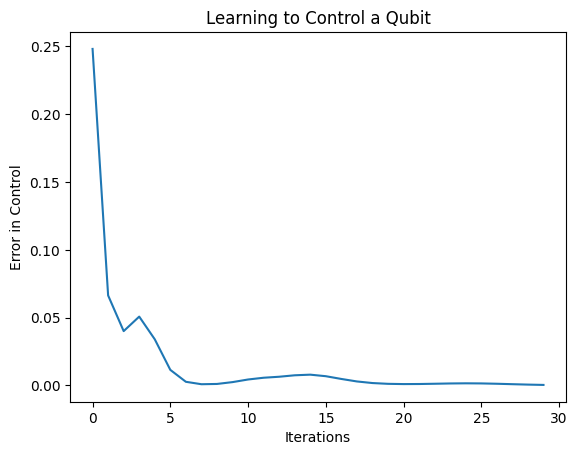
損失関数はゼロに低下しました。
controllerはスタンドアロンモデルとして利用できます。コントローラを呼び出し、各コマンド信号に対する応答を確認します。これらの出力をrandom_rotationsの内容と正しく比較するには、ある程度の作業が必要になります。
controller.predict(np.array([0,1]))
array([[3.6335812 , 1.8470774 , 0.71675825],
       [5.3085413 , 0.08116499, 2.8337662 ]], dtype=float32)