
|
|
|
 View on GitHub View on GitHub
|
|
Introduction
Decision Forests (DF) are a family of Machine Learning algorithms for supervised classification, regression and ranking. As the name suggests, DFs use decision trees as a building block. Today, the two most popular DF training algorithms are Random Forests and Gradient Boosted Decision Trees.
TensorFlow Decision Forests (TF-DF) is a library for the training, evaluation, interpretation and inference of Decision Forest models.
In this tutorial, you will learn how to:
- Train a multi-class classification Random Forest on a dataset containing numerical, categorical and missing features.
- Evaluate the model on a test dataset.
- Prepare the model for TensorFlow Serving.
- Examine the overall structure of the model and the importance of each feature.
- Re-train the model with a different learning algorithm (Gradient Boosted Decision Trees).
- Use a different set of input features.
- Change the hyperparameters of the model.
- Preprocess the features.
- Train a model for regression.
Detailed documentation is available in the user manual. The example directory contains other end-to-end examples.
Installing TensorFlow Decision Forests
Install TF-DF by running the following cell.
pip install tensorflow_decision_forestsWurlitzer is needed to display the detailed training logs in Colabs (when using verbose=2 in the model constructor).
pip install wurlitzerImporting libraries
import os
# Keep using Keras 2
os.environ['TF_USE_LEGACY_KERAS'] = '1'

import tensorflow_decision_forests as tfdf

import numpy as np
import pandas as pd
import tensorflow as tf
import tf_keras
import math
2026-01-12 13:59:46.395546: E external/local_xla/xla/stream_executor/cuda/cuda_fft.cc:467] Unable to register cuFFT factory: Attempting to register factory for plugin cuFFT when one has already been registered
WARNING: All log messages before absl::InitializeLog() is called are written to STDERR
E0000 00:00:1768226386.418824   10462 cuda_dnn.cc:8579] Unable to register cuDNN factory: Attempting to register factory for plugin cuDNN when one has already been registered
E0000 00:00:1768226386.426729   10462 cuda_blas.cc:1407] Unable to register cuBLAS factory: Attempting to register factory for plugin cuBLAS when one has already been registered
W0000 00:00:1768226386.445654   10462 computation_placer.cc:177] computation placer already registered. Please check linkage and avoid linking the same target more than once.
W0000 00:00:1768226386.445674   10462 computation_placer.cc:177] computation placer already registered. Please check linkage and avoid linking the same target more than once.
W0000 00:00:1768226386.445677   10462 computation_placer.cc:177] computation placer already registered. Please check linkage and avoid linking the same target more than once.
W0000 00:00:1768226386.445679   10462 computation_placer.cc:177] computation placer already registered. Please check linkage and avoid linking the same target more than once.
The hidden code cell limits the output height in colab.
from IPython.core.magic import register_line_magic
from IPython.display import Javascript
from IPython.display import display as ipy_display

# Some of the model training logs can cover the full
# screen if not compressed to a smaller viewport.
# This magic allows setting a max height for a cell.
@register_line_magic
def set_cell_height(size):
  ipy_display(
      Javascript("google.colab.output.setIframeHeight(0, true, {maxHeight: " +
                 str(size) + "})"))
# Check the version of TensorFlow Decision Forests
print("Found TensorFlow Decision Forests v" + tfdf.__version__)
Found TensorFlow Decision Forests v1.12.0
Training a Random Forest model
In this section, we train, evaluate, analyse and export a multi-class classification Random Forest trained on the Palmer's Penguins dataset.

Load the dataset and convert it in a tf.Dataset
This dataset is very small (300 examples) and stored as a .csv-like file. Therefore, use Pandas to load it.
Let's assemble the dataset into a csv file (i.e. add the header), and load it:
# Download the dataset
!wget -q https://storage.googleapis.com/download.tensorflow.org/data/palmer_penguins/penguins.csv -O /tmp/penguins.csv

# Load a dataset into a Pandas Dataframe.
dataset_df = pd.read_csv("/tmp/penguins.csv")

# Display the first 3 examples.
dataset_df.head(3)
The dataset contains a mix of numerical (e.g. bill_depth_mm), categorical
(e.g. island) and missing features. TF-DF supports all these feature types natively (differently than NN based models), therefore there is no need for preprocessing in the form of one-hot encoding, normalization or extra is_present feature.
Labels are a bit different: Keras metrics expect integers. The label (species) is stored as a string, so let's convert it into an integer.
# Encode the categorical labels as integers.
#
# Details:
# This stage is necessary if your classification label is represented as a
# string since Keras expects integer classification labels.
# When using `pd_dataframe_to_tf_dataset` (see below), this step can be skipped.

# Name of the label column.
label = "species"

classes = dataset_df[label].unique().tolist()
print(f"Label classes: {classes}")

dataset_df[label] = dataset_df[label].map(classes.index)
Label classes: ['Adelie', 'Gentoo', 'Chinstrap']
Next split the dataset into training and testing:
# Split the dataset into a training and a testing dataset.

def split_dataset(dataset, test_ratio=0.30):
  """Splits a panda dataframe in two."""
  test_indices = np.random.rand(len(dataset)) < test_ratio
  return dataset[~test_indices], dataset[test_indices]


train_ds_pd, test_ds_pd = split_dataset(dataset_df)
print("{} examples in training, {} examples for testing.".format(
    len(train_ds_pd), len(test_ds_pd)))
250 examples in training, 94 examples for testing.
And finally, convert the pandas dataframe (pd.Dataframe) into tensorflow datasets (tf.data.Dataset):
train_ds = tfdf.keras.pd_dataframe_to_tf_dataset(train_ds_pd, label=label)
test_ds = tfdf.keras.pd_dataframe_to_tf_dataset(test_ds_pd, label=label)
I0000 00:00:1768226390.702906   10462 gpu_device.cc:2019] Created device /job:localhost/replica:0/task:0/device:GPU:0 with 13638 MB memory:  -> device: 0, name: Tesla T4, pci bus id: 0000:00:05.0, compute capability: 7.5
I0000 00:00:1768226390.705145   10462 gpu_device.cc:2019] Created device /job:localhost/replica:0/task:0/device:GPU:1 with 13756 MB memory:  -> device: 1, name: Tesla T4, pci bus id: 0000:00:06.0, compute capability: 7.5
I0000 00:00:1768226390.707437   10462 gpu_device.cc:2019] Created device /job:localhost/replica:0/task:0/device:GPU:2 with 13756 MB memory:  -> device: 2, name: Tesla T4, pci bus id: 0000:00:07.0, compute capability: 7.5
I0000 00:00:1768226390.709568   10462 gpu_device.cc:2019] Created device /job:localhost/replica:0/task:0/device:GPU:3 with 13756 MB memory:  -> device: 3, name: Tesla T4, pci bus id: 0000:00:08.0, compute capability: 7.5
Notes: Recall that pd_dataframe_to_tf_dataset converts string labels to integers if necessary.
If you want to create the tf.data.Dataset yourself, there are a couple of things to remember:
- The learning algorithms work with a one-epoch dataset and without shuffling.
- The batch size does not impact the training algorithm, but a small value might slow down reading the dataset.
Train the model
%set_cell_height 300

# Specify the model.
model_1 = tfdf.keras.RandomForestModel(verbose=2)

# Train the model.
model_1.fit(train_ds)
<IPython.core.display.Javascript object>
Warning: The `num_threads` constructor argument is not set and the number of CPU is os.cpu_count()=32 > 32. Setting num_threads to 32. Set num_threads manually to use more than 32 cpus.
WARNING:absl:The `num_threads` constructor argument is not set and the number of CPU is os.cpu_count()=32 > 32. Setting num_threads to 32. Set num_threads manually to use more than 32 cpus.
Use /tmpfs/tmp/tmpauvzz185 as temporary training directory
Reading training dataset...
Training tensor examples:
Features: {'island': <tf.Tensor 'data:0' shape=(None,) dtype=string>, 'bill_length_mm': <tf.Tensor 'data_1:0' shape=(None,) dtype=float64>, 'bill_depth_mm': <tf.Tensor 'data_2:0' shape=(None,) dtype=float64>, 'flipper_length_mm': <tf.Tensor 'data_3:0' shape=(None,) dtype=float64>, 'body_mass_g': <tf.Tensor 'data_4:0' shape=(None,) dtype=float64>, 'sex': <tf.Tensor 'data_5:0' shape=(None,) dtype=string>, 'year': <tf.Tensor 'data_6:0' shape=(None,) dtype=int64>}
Label: Tensor("data_7:0", shape=(None,), dtype=int64)
Weights: None
Normalized tensor features:
 {'island': SemanticTensor(semantic=<Semantic.CATEGORICAL: 2>, tensor=<tf.Tensor 'data:0' shape=(None,) dtype=string>), 'bill_length_mm': SemanticTensor(semantic=<Semantic.NUMERICAL: 1>, tensor=<tf.Tensor 'Cast:0' shape=(None,) dtype=float32>), 'bill_depth_mm': SemanticTensor(semantic=<Semantic.NUMERICAL: 1>, tensor=<tf.Tensor 'Cast_1:0' shape=(None,) dtype=float32>), 'flipper_length_mm': SemanticTensor(semantic=<Semantic.NUMERICAL: 1>, tensor=<tf.Tensor 'Cast_2:0' shape=(None,) dtype=float32>), 'body_mass_g': SemanticTensor(semantic=<Semantic.NUMERICAL: 1>, tensor=<tf.Tensor 'Cast_3:0' shape=(None,) dtype=float32>), 'sex': SemanticTensor(semantic=<Semantic.CATEGORICAL: 2>, tensor=<tf.Tensor 'data_5:0' shape=(None,) dtype=string>), 'year': SemanticTensor(semantic=<Semantic.NUMERICAL: 1>, tensor=<tf.Tensor 'Cast_4:0' shape=(None,) dtype=float32>)}
Training dataset read in 0:00:03.851266. Found 250 examples.
Training model...
Standard output detected as not visible to the user e.g. running in a notebook. Creating a training log redirection. If training gets stuck, try calling tfdf.keras.set_training_logs_redirection(False).
Model trained in 0:00:00.058962
Compiling model...
Model compiled.
<tf_keras.src.callbacks.History at 0x7f85d804e670>
Remarks
- No input features are specified. Therefore, all the columns will be used as
input features except for the label. The feature used by the model are shown
in the training logs and in the
model.summary(). - DFs consume natively numerical, categorical, categorical-set features and missing-values. Numerical features do not need to be normalized. Categorical string values do not need to be encoded in a dictionary.
- No training hyper-parameters are specified. Therefore the default hyper-parameters will be used. Default hyper-parameters provide reasonable results in most situations.
- Calling
compileon the model before thefitis optional. Compile can be used to provide extra evaluation metrics. - Training algorithms do not need validation datasets. If a validation dataset is provided, it will only be used to show metrics.
- Tweak the
verboseargument toRandomForestModelto control the amount of displayed training logs. Setverbose=0to hide most of the logs. Setverbose=2to show all the logs.
Evaluate the model
Let's evaluate our model on the test dataset.
model_1.compile(metrics=["accuracy"])
evaluation = model_1.evaluate(test_ds, return_dict=True)
print()

for name, value in evaluation.items():
  print(f"{name}: {value:.4f}")
1/1 [==============================] - 0s 290ms/step - loss: 0.0000e+00 - accuracy: 1.0000

loss: 0.0000
accuracy: 1.0000
Remark: The test accuracy is close to the Out-of-bag accuracy shown in the training logs.
See the Model Self Evaluation section below for more evaluation methods.
Prepare this model for TensorFlow Serving.
Export the model to the SavedModel format for later re-use e.g. TensorFlow Serving.
model_1.save("/tmp/my_saved_model")
INFO:tensorflow:Assets written to: /tmp/my_saved_model/assets
INFO:tensorflow:Assets written to: /tmp/my_saved_model/assets
Plot the model
Plotting a decision tree and following the first branches helps learning about decision forests. In some cases, plotting a model can even be used for debugging.
Because of the difference in the way they are trained, some models are more interesting to plan than others. Because of the noise injected during training and the depth of the trees, plotting Random Forest is less informative than plotting a CART or the first tree of a Gradient Boosted Tree.
Never the less, let's plot the first tree of our Random Forest model:
tfdf.model_plotter.plot_model_in_colab(model_1, tree_idx=0, max_depth=3)
The root node on the left contains the first condition (bill_depth_mm >= 16.55), number of examples (240) and label distribution (the red-blue-green bar).
Examples that evaluates true to bill_depth_mm >= 16.55 are branched to the green path. The other ones are branched to the red path.
The deeper the node, the more pure they become i.e. the label distribution is biased toward a subset of classes.
Model structure and feature importance
The overall structure of the model is show with .summary(). You will see:
- Type: The learning algorithm used to train the model (
Random Forestin our case). - Task: The problem solved by the model (
Classificationin our case). - Input Features: The input features of the model.
- Variable Importance: Different measures of the importance of each feature for the model.
- Out-of-bag evaluation: The out-of-bag evaluation of the model. This is a cheap and efficient alternative to cross-validation.
- Number of {trees, nodes} and other metrics: Statistics about the structure of the decisions forests.
Remark: The summary's content depends on the learning algorithm (e.g. Out-of-bag is only available for Random Forest) and the hyper-parameters (e.g. the mean-decrease-in-accuracy variable importance can be disabled in the hyper-parameters).
%set_cell_height 300
model_1.summary()
<IPython.core.display.Javascript object>
Model: "random_forest_model"
_________________________________________________________________
 Layer (type)                Output Shape              Param #
=================================================================
=================================================================
Total params: 1 (1.00 Byte)
Trainable params: 0 (0.00 Byte)
Non-trainable params: 1 (1.00 Byte)
_________________________________________________________________
Type: "RANDOM_FOREST"
Task: CLASSIFICATION
Label: "__LABEL"

Input Features (7):
    bill_depth_mm
    bill_length_mm
    body_mass_g
    flipper_length_mm
    island
    sex
    year

No weights

Variable Importance: INV_MEAN_MIN_DEPTH:

    1. "flipper_length_mm"  0.435977 ################
    2.    "bill_length_mm"  0.396917 ############
    3.     "bill_depth_mm"  0.327861 #######
    4.            "island"  0.309749 ######
    5.       "body_mass_g"  0.258320 ##
    6.               "sex"  0.234113
    7.              "year"  0.231849

Variable Importance: NUM_AS_ROOT:

    1. "flipper_length_mm" 151.000000 ################
    2.     "bill_depth_mm" 75.000000 #######
    3.    "bill_length_mm" 58.000000 #####
    4.            "island" 13.000000 #
    5.       "body_mass_g"  3.000000

Variable Importance: NUM_NODES:

    1.    "bill_length_mm" 707.000000 ################
    2.     "bill_depth_mm" 416.000000 #########
    3. "flipper_length_mm" 394.000000 ########
    4.            "island" 297.000000 ######
    5.       "body_mass_g" 290.000000 ######
    6.               "sex" 52.000000
    7.              "year" 19.000000

Variable Importance: SUM_SCORE:

    1. "flipper_length_mm" 24627.319999 ################
    2.    "bill_length_mm" 24086.337571 ###############
    3.     "bill_depth_mm" 14073.983456 #########
    4.            "island" 10081.743781 ######
    5.       "body_mass_g" 2495.079835 #
    6.               "sex" 442.453467
    7.              "year" 56.784963


Winner takes all: true
Out-of-bag evaluation: accuracy:0.98 logloss:0.0970684
Number of trees: 300
Total number of nodes: 4650

Number of nodes by tree:
Count: 300 Average: 15.5 StdDev: 3.15859
Min: 9 Max: 27 Ignored: 0
----------------------------------------------
[  9, 10)  1   0.33%   0.33%
[ 10, 11)  0   0.00%   0.33%
[ 11, 12) 29   9.67%  10.00% ###
[ 12, 13)  0   0.00%  10.00%
[ 13, 14) 72  24.00%  34.00% ########
[ 14, 15)  0   0.00%  34.00%
[ 15, 16) 94  31.33%  65.33% ##########
[ 16, 17)  0   0.00%  65.33%
[ 17, 18) 48  16.00%  81.33% #####
[ 18, 19)  0   0.00%  81.33%
[ 19, 20) 28   9.33%  90.67% ###
[ 20, 21)  0   0.00%  90.67%
[ 21, 22) 15   5.00%  95.67% ##
[ 22, 23)  0   0.00%  95.67%
[ 23, 24)  8   2.67%  98.33% #
[ 24, 25)  0   0.00%  98.33%
[ 25, 26)  3   1.00%  99.33%
[ 26, 27)  0   0.00%  99.33%
[ 27, 27]  2   0.67% 100.00%

Depth by leafs:
Count: 2475 Average: 3.41293 StdDev: 1.08618
Min: 1 Max: 7 Ignored: 0
----------------------------------------------
[ 1, 2)   5   0.20%   0.20%
[ 2, 3) 599  24.20%  24.40% ########
[ 3, 4) 711  28.73%  53.13% #########
[ 4, 5) 754  30.46%  83.60% ##########
[ 5, 6) 351  14.18%  97.78% #####
[ 6, 7)  45   1.82%  99.60% #
[ 7, 7]  10   0.40% 100.00%

Number of training obs by leaf:
Count: 2475 Average: 30.303 StdDev: 32.0454
Min: 5 Max: 112 Ignored: 0
----------------------------------------------
[   5,  10) 1257  50.79%  50.79% ##########
[  10,  15)  120   4.85%  55.64% #
[  15,  21)   79   3.19%  58.83% #
[  21,  26)   59   2.38%  61.21%
[  26,  32)   88   3.56%  64.77% #
[  32,  37)   66   2.67%  67.43% #
[  37,  42)   74   2.99%  70.42% #
[  42,  48)   76   3.07%  73.49% #
[  48,  53)   53   2.14%  75.64%
[  53,  59)   32   1.29%  76.93%
[  59,  64)   31   1.25%  78.18%
[  64,  69)   42   1.70%  79.88%
[  69,  75)   56   2.26%  82.14%
[  75,  80)   61   2.46%  84.61%
[  80,  86)  113   4.57%  89.17% #
[  86,  91)  105   4.24%  93.41% #
[  91,  96)   77   3.11%  96.53% #
[  96, 102)   63   2.55%  99.07% #
[ 102, 107)   18   0.73%  99.80%
[ 107, 112]    5   0.20% 100.00%

Attribute in nodes:
    707 : bill_length_mm [NUMERICAL]
    416 : bill_depth_mm [NUMERICAL]
    394 : flipper_length_mm [NUMERICAL]
    297 : island [CATEGORICAL]
    290 : body_mass_g [NUMERICAL]
    52 : sex [CATEGORICAL]
    19 : year [NUMERICAL]

Attribute in nodes with depth <= 0:
    151 : flipper_length_mm [NUMERICAL]
    75 : bill_depth_mm [NUMERICAL]
    58 : bill_length_mm [NUMERICAL]
    13 : island [CATEGORICAL]
    3 : body_mass_g [NUMERICAL]

Attribute in nodes with depth <= 1:
    250 : flipper_length_mm [NUMERICAL]
    223 : bill_length_mm [NUMERICAL]
    206 : bill_depth_mm [NUMERICAL]
    152 : island [CATEGORICAL]
    63 : body_mass_g [NUMERICAL]
    1 : year [NUMERICAL]

Attribute in nodes with depth <= 2:
    437 : bill_length_mm [NUMERICAL]
    329 : flipper_length_mm [NUMERICAL]
    299 : bill_depth_mm [NUMERICAL]
    249 : island [CATEGORICAL]
    160 : body_mass_g [NUMERICAL]
    9 : sex [CATEGORICAL]
    3 : year [NUMERICAL]

Attribute in nodes with depth <= 3:
    619 : bill_length_mm [NUMERICAL]
    381 : bill_depth_mm [NUMERICAL]
    370 : flipper_length_mm [NUMERICAL]
    289 : island [CATEGORICAL]
    249 : body_mass_g [NUMERICAL]
    38 : sex [CATEGORICAL]
    11 : year [NUMERICAL]

Attribute in nodes with depth <= 5:
    704 : bill_length_mm [NUMERICAL]
    414 : bill_depth_mm [NUMERICAL]
    394 : flipper_length_mm [NUMERICAL]
    297 : island [CATEGORICAL]
    290 : body_mass_g [NUMERICAL]
    52 : sex [CATEGORICAL]
    19 : year [NUMERICAL]

Condition type in nodes:
    1826 : HigherCondition
    349 : ContainsBitmapCondition
Condition type in nodes with depth <= 0:
    287 : HigherCondition
    13 : ContainsBitmapCondition
Condition type in nodes with depth <= 1:
    743 : HigherCondition
    152 : ContainsBitmapCondition
Condition type in nodes with depth <= 2:
    1228 : HigherCondition
    258 : ContainsBitmapCondition
Condition type in nodes with depth <= 3:
    1630 : HigherCondition
    327 : ContainsBitmapCondition
Condition type in nodes with depth <= 5:
    1821 : HigherCondition
    349 : ContainsBitmapCondition
Node format: NOT_SET

Training OOB:
    trees: 1, Out-of-bag evaluation: accuracy:0.947917 logloss:1.87727
    trees: 11, Out-of-bag evaluation: accuracy:0.943775 logloss:0.660757
    trees: 21, Out-of-bag evaluation: accuracy:0.968 logloss:0.506145
    trees: 31, Out-of-bag evaluation: accuracy:0.956 logloss:0.241419
    trees: 42, Out-of-bag evaluation: accuracy:0.956 logloss:0.240549
    trees: 52, Out-of-bag evaluation: accuracy:0.964 logloss:0.234582
    trees: 63, Out-of-bag evaluation: accuracy:0.964 logloss:0.23867
    trees: 73, Out-of-bag evaluation: accuracy:0.972 logloss:0.235637
    trees: 83, Out-of-bag evaluation: accuracy:0.972 logloss:0.232233
    trees: 93, Out-of-bag evaluation: accuracy:0.972 logloss:0.228022
    trees: 103, Out-of-bag evaluation: accuracy:0.976 logloss:0.0953604
    trees: 114, Out-of-bag evaluation: accuracy:0.972 logloss:0.0925293
    trees: 124, Out-of-bag evaluation: accuracy:0.976 logloss:0.0922547
    trees: 134, Out-of-bag evaluation: accuracy:0.976 logloss:0.0932468
    trees: 144, Out-of-bag evaluation: accuracy:0.976 logloss:0.0949779
    trees: 154, Out-of-bag evaluation: accuracy:0.976 logloss:0.0958475
    trees: 165, Out-of-bag evaluation: accuracy:0.976 logloss:0.096324
    trees: 175, Out-of-bag evaluation: accuracy:0.976 logloss:0.0955369
    trees: 186, Out-of-bag evaluation: accuracy:0.98 logloss:0.0917101
    trees: 196, Out-of-bag evaluation: accuracy:0.98 logloss:0.091533
    trees: 208, Out-of-bag evaluation: accuracy:0.98 logloss:0.092786
    trees: 218, Out-of-bag evaluation: accuracy:0.98 logloss:0.092438
    trees: 228, Out-of-bag evaluation: accuracy:0.98 logloss:0.0941152
    trees: 238, Out-of-bag evaluation: accuracy:0.98 logloss:0.0955081
    trees: 249, Out-of-bag evaluation: accuracy:0.98 logloss:0.0950918
    trees: 259, Out-of-bag evaluation: accuracy:0.98 logloss:0.0952201
    trees: 269, Out-of-bag evaluation: accuracy:0.98 logloss:0.0941477
    trees: 279, Out-of-bag evaluation: accuracy:0.98 logloss:0.0946589
    trees: 289, Out-of-bag evaluation: accuracy:0.98 logloss:0.0960823
    trees: 299, Out-of-bag evaluation: accuracy:0.98 logloss:0.0960505
    trees: 300, Out-of-bag evaluation: accuracy:0.98 logloss:0.0970684
The information in summary are all available programmatically using the model inspector:
# The input features
model_1.make_inspector().features()
["bill_depth_mm" (1; #1),
 "bill_length_mm" (1; #2),
 "body_mass_g" (1; #3),
 "flipper_length_mm" (1; #4),
 "island" (4; #5),
 "sex" (4; #6),
 "year" (1; #7)]
# The feature importances
model_1.make_inspector().variable_importances()
{'INV_MEAN_MIN_DEPTH': [("flipper_length_mm" (1; #4), 0.43597672269512794),
  ("bill_length_mm" (1; #2), 0.3969174550696071),
  ("bill_depth_mm" (1; #1), 0.3278611602910266),
  ("island" (4; #5), 0.3097488348618274),
  ("body_mass_g" (1; #3), 0.25832019126054884),
  ("sex" (4; #6), 0.23411343302569165),
  ("year" (1; #7), 0.23184865027854668)],
 'SUM_SCORE': [("flipper_length_mm" (1; #4), 24627.319999137893),
  ("bill_length_mm" (1; #2), 24086.33757083863),
  ("bill_depth_mm" (1; #1), 14073.983455628157),
  ("island" (4; #5), 10081.743780997582),
  ("body_mass_g" (1; #3), 2495.07983523421),
  ("sex" (4; #6), 442.45346712321043),
  ("year" (1; #7), 56.7849625647068)],
 'NUM_AS_ROOT': [("flipper_length_mm" (1; #4), 151.0),
  ("bill_depth_mm" (1; #1), 75.0),
  ("bill_length_mm" (1; #2), 58.0),
  ("island" (4; #5), 13.0),
  ("body_mass_g" (1; #3), 3.0)],
 'NUM_NODES': [("bill_length_mm" (1; #2), 707.0),
  ("bill_depth_mm" (1; #1), 416.0),
  ("flipper_length_mm" (1; #4), 394.0),
  ("island" (4; #5), 297.0),
  ("body_mass_g" (1; #3), 290.0),
  ("sex" (4; #6), 52.0),
  ("year" (1; #7), 19.0)]}
The content of the summary and the inspector depends on the learning algorithm (tfdf.keras.RandomForestModel in this case) and its hyper-parameters (e.g. compute_oob_variable_importances=True will trigger the computation of Out-of-bag variable importances for the Random Forest learner).
Model Self Evaluation
During training TFDF models can self evaluate even if no validation dataset is provided to the fit() method. The exact logic depends on the model. For example, Random Forest will use Out-of-bag evaluation while Gradient Boosted Trees will use internal train-validation.
The model self evaluation is available with the inspector's evaluation():
model_1.make_inspector().evaluation()
Evaluation(num_examples=250, accuracy=0.98, loss=0.09706837522983551, rmse=None, ndcg=None, aucs=None, auuc=None, qini=None)
Plotting the training logs
The training logs show the quality of the model (e.g. accuracy evaluated on the out-of-bag or validation dataset) according to the number of trees in the model. These logs are helpful to study the balance between model size and model quality.
The logs are available in multiple ways:
- Displayed in during training if
fit()is wrapped inwith sys_pipes():(see example above). - At the end of the model summary i.e.
model.summary()(see example above). - Programmatically, using the model inspector i.e.
model.make_inspector().training_logs(). - Using TensorBoard
Let's try the options 2 and 3:
%set_cell_height 150
model_1.make_inspector().training_logs()
<IPython.core.display.Javascript object>
[TrainLog(num_trees=1, evaluation=Evaluation(num_examples=96, accuracy=0.9479166666666666, loss=1.8772735198338826, rmse=None, ndcg=None, aucs=None, auuc=None, qini=None)),
 TrainLog(num_trees=11, evaluation=Evaluation(num_examples=249, accuracy=0.9437751004016064, loss=0.6607572125143795, rmse=None, ndcg=None, aucs=None, auuc=None, qini=None)),
 TrainLog(num_trees=21, evaluation=Evaluation(num_examples=250, accuracy=0.968, loss=0.506145211815834, rmse=None, ndcg=None, aucs=None, auuc=None, qini=None)),
 TrainLog(num_trees=31, evaluation=Evaluation(num_examples=250, accuracy=0.956, loss=0.24141885021328927, rmse=None, ndcg=None, aucs=None, auuc=None, qini=None)),
 TrainLog(num_trees=42, evaluation=Evaluation(num_examples=250, accuracy=0.956, loss=0.2405486009567976, rmse=None, ndcg=None, aucs=None, auuc=None, qini=None)),
 TrainLog(num_trees=52, evaluation=Evaluation(num_examples=250, accuracy=0.964, loss=0.23458186860382557, rmse=None, ndcg=None, aucs=None, auuc=None, qini=None)),
 TrainLog(num_trees=63, evaluation=Evaluation(num_examples=250, accuracy=0.964, loss=0.23867048719525338, rmse=None, ndcg=None, aucs=None, auuc=None, qini=None)),
 TrainLog(num_trees=73, evaluation=Evaluation(num_examples=250, accuracy=0.972, loss=0.2356372931599617, rmse=None, ndcg=None, aucs=None, auuc=None, qini=None)),
 TrainLog(num_trees=83, evaluation=Evaluation(num_examples=250, accuracy=0.972, loss=0.2322330457419157, rmse=None, ndcg=None, aucs=None, auuc=None, qini=None)),
 TrainLog(num_trees=93, evaluation=Evaluation(num_examples=250, accuracy=0.972, loss=0.22802215158939362, rmse=None, ndcg=None, aucs=None, auuc=None, qini=None)),
 TrainLog(num_trees=103, evaluation=Evaluation(num_examples=250, accuracy=0.976, loss=0.0953604139611125, rmse=None, ndcg=None, aucs=None, auuc=None, qini=None)),
 TrainLog(num_trees=114, evaluation=Evaluation(num_examples=250, accuracy=0.972, loss=0.09252933283150196, rmse=None, ndcg=None, aucs=None, auuc=None, qini=None)),
 TrainLog(num_trees=124, evaluation=Evaluation(num_examples=250, accuracy=0.976, loss=0.0922547305226326, rmse=None, ndcg=None, aucs=None, auuc=None, qini=None)),
 TrainLog(num_trees=134, evaluation=Evaluation(num_examples=250, accuracy=0.976, loss=0.09324676994979382, rmse=None, ndcg=None, aucs=None, auuc=None, qini=None)),
 TrainLog(num_trees=144, evaluation=Evaluation(num_examples=250, accuracy=0.976, loss=0.09497785523533821, rmse=None, ndcg=None, aucs=None, auuc=None, qini=None)),
 TrainLog(num_trees=154, evaluation=Evaluation(num_examples=250, accuracy=0.976, loss=0.09584752155095339, rmse=None, ndcg=None, aucs=None, auuc=None, qini=None)),
 TrainLog(num_trees=165, evaluation=Evaluation(num_examples=250, accuracy=0.976, loss=0.09632397620007396, rmse=None, ndcg=None, aucs=None, auuc=None, qini=None)),
 TrainLog(num_trees=175, evaluation=Evaluation(num_examples=250, accuracy=0.976, loss=0.09553687626868486, rmse=None, ndcg=None, aucs=None, auuc=None, qini=None)),
 TrainLog(num_trees=186, evaluation=Evaluation(num_examples=250, accuracy=0.98, loss=0.09171005741134286, rmse=None, ndcg=None, aucs=None, auuc=None, qini=None)),
 TrainLog(num_trees=196, evaluation=Evaluation(num_examples=250, accuracy=0.98, loss=0.09153303373605012, rmse=None, ndcg=None, aucs=None, auuc=None, qini=None)),
 TrainLog(num_trees=208, evaluation=Evaluation(num_examples=250, accuracy=0.98, loss=0.09278595473244786, rmse=None, ndcg=None, aucs=None, auuc=None, qini=None)),
 TrainLog(num_trees=218, evaluation=Evaluation(num_examples=250, accuracy=0.98, loss=0.09243803822994232, rmse=None, ndcg=None, aucs=None, auuc=None, qini=None)),
 TrainLog(num_trees=228, evaluation=Evaluation(num_examples=250, accuracy=0.98, loss=0.09411523111537098, rmse=None, ndcg=None, aucs=None, auuc=None, qini=None)),
 TrainLog(num_trees=238, evaluation=Evaluation(num_examples=250, accuracy=0.98, loss=0.0955081114768982, rmse=None, ndcg=None, aucs=None, auuc=None, qini=None)),
 TrainLog(num_trees=249, evaluation=Evaluation(num_examples=250, accuracy=0.98, loss=0.09509177429974079, rmse=None, ndcg=None, aucs=None, auuc=None, qini=None)),
 TrainLog(num_trees=259, evaluation=Evaluation(num_examples=250, accuracy=0.98, loss=0.0952201502174139, rmse=None, ndcg=None, aucs=None, auuc=None, qini=None)),
 TrainLog(num_trees=269, evaluation=Evaluation(num_examples=250, accuracy=0.98, loss=0.0941477091498673, rmse=None, ndcg=None, aucs=None, auuc=None, qini=None)),
 TrainLog(num_trees=279, evaluation=Evaluation(num_examples=250, accuracy=0.98, loss=0.09465892957895994, rmse=None, ndcg=None, aucs=None, auuc=None, qini=None)),
 TrainLog(num_trees=289, evaluation=Evaluation(num_examples=250, accuracy=0.98, loss=0.09608231737092138, rmse=None, ndcg=None, aucs=None, auuc=None, qini=None)),
 TrainLog(num_trees=299, evaluation=Evaluation(num_examples=250, accuracy=0.98, loss=0.09605051735416055, rmse=None, ndcg=None, aucs=None, auuc=None, qini=None)),
 TrainLog(num_trees=300, evaluation=Evaluation(num_examples=250, accuracy=0.98, loss=0.09706837522983551, rmse=None, ndcg=None, aucs=None, auuc=None, qini=None))]
Let's plot it:
import matplotlib.pyplot as plt

logs = model_1.make_inspector().training_logs()

plt.figure(figsize=(12, 4))

plt.subplot(1, 2, 1)
plt.plot([log.num_trees for log in logs], [log.evaluation.accuracy for log in logs])
plt.xlabel("Number of trees")
plt.ylabel("Accuracy (out-of-bag)")

plt.subplot(1, 2, 2)
plt.plot([log.num_trees for log in logs], [log.evaluation.loss for log in logs])
plt.xlabel("Number of trees")
plt.ylabel("Logloss (out-of-bag)")

plt.show()
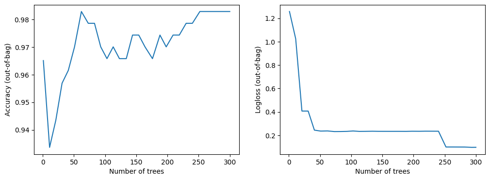
This dataset is small. You can see the model converging almost immediately.
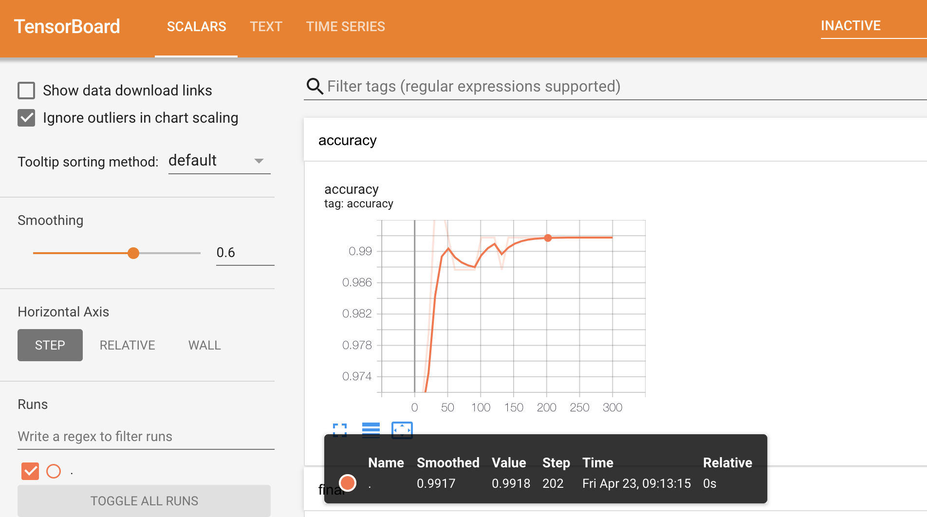
Let's use TensorBoard:
# This cell start TensorBoard that can be slow.
# Load the TensorBoard notebook extension
%load_ext tensorboard
# Google internal version
# %load_ext google3.learning.brain.tensorboard.notebook.extension
# Clear existing results (if any)rm -fr "/tmp/tensorboard_logs"
# Export the meta-data to tensorboard.
model_1.make_inspector().export_to_tensorboard("/tmp/tensorboard_logs")
# docs_infra: no_execute
# Start a tensorboard instance.
%tensorboard --logdir "/tmp/tensorboard_logs"
Re-train the model with a different learning algorithm
The learning algorithm is defined by the model class. For
example, tfdf.keras.RandomForestModel() trains a Random Forest, while
tfdf.keras.GradientBoostedTreesModel() trains a Gradient Boosted Decision
Trees.
The learning algorithms are listed by calling tfdf.keras.get_all_models() or in the
learner list.
tfdf.keras.get_all_models()
[tensorflow_decision_forests.keras.RandomForestModel,
 tensorflow_decision_forests.keras.GradientBoostedTreesModel,
 tensorflow_decision_forests.keras.CartModel,
 tensorflow_decision_forests.keras.DistributedGradientBoostedTreesModel]
The description of the learning algorithms and their hyper-parameters are also available in the API reference and builtin help:
# help works anywhere.
help(tfdf.keras.RandomForestModel)

# ? only works in ipython or notebooks, it usually opens on a separate panel.
tfdf.keras.RandomForestModel?
Help on class RandomForestModel in module tensorflow_decision_forests.keras:
class RandomForestModel(tensorflow_decision_forests.keras.wrappers.RandomForestModel)
| RandomForestModel(*args, **kwargs)
|
| Method resolution order:
| RandomForestModel
| tensorflow_decision_forests.keras.wrappers.RandomForestModel
| tensorflow_decision_forests.keras.core.CoreModel
| tensorflow_decision_forests.keras.core_inference.InferenceCoreModel
| tf_keras.src.engine.training.Model
| tf_keras.src.engine.base_layer.Layer
| tensorflow.python.module.module.Module
| tensorflow.python.trackable.autotrackable.AutoTrackable
| tensorflow.python.trackable.base.Trackable
| tf_keras.src.utils.version_utils.LayerVersionSelector
| tf_keras.src.utils.version_utils.ModelVersionSelector
| builtins.object
|
| Methods inherited from tensorflow_decision_forests.keras.wrappers.RandomForestModel:
|
| __init__(self, task: Optional[ForwardRef('abstract_model_pb2.Task')] = 1, features: Optional[List[tensorflow_decision_forests.keras.core.FeatureUsage]] = None, exclude_non_specified_features: Optional[bool] = False, preprocessing: Optional[ForwardRef('tf_keras.models.Functional')] = None, postprocessing: Optional[ForwardRef('tf_keras.models.Functional')] = None, training_preprocessing: Optional[ForwardRef('tf_keras.models.Functional')] = None, ranking_group: Optional[str] = None, uplift_treatment: Optional[str] = None, temp_directory: Optional[str] = None, verbose: int = 1, hyperparameter_template: Optional[str] = None, advanced_arguments: Optional[tensorflow_decision_forests.keras.core_inference.AdvancedArguments] = None, num_threads: Optional[int] = None, name: Optional[str] = None, max_vocab_count: Optional[int] = 2000, try_resume_training: Optional[bool] = True, check_dataset: Optional[bool] = True, tuner: Optional[tensorflow_decision_forests.component.tuner.tuner.Tuner] = None, discretize_numerical_features: bool = False, num_discretized_numerical_bins: int = 255, multitask: Optional[List[tensorflow_decision_forests.keras.core_inference.MultiTaskItem]] = None, adapt_bootstrap_size_ratio_for_maximum_training_duration: Optional[bool] = False, allow_na_conditions: Optional[bool] = False, bootstrap_size_ratio: Optional[float] = 1.0, bootstrap_training_dataset: Optional[bool] = True, categorical_algorithm: Optional[str] = 'CART', categorical_set_split_greedy_sampling: Optional[float] = 0.1, categorical_set_split_max_num_items: Optional[int] = -1, categorical_set_split_min_item_frequency: Optional[int] = 1, compute_oob_performances: Optional[bool] = True, compute_oob_variable_importances: Optional[bool] = False, growing_strategy: Optional[str] = 'LOCAL', honest: Optional[bool] = False, honest_fixed_separation: Optional[bool] = False, honest_ratio_leaf_examples: Optional[float] = 0.5, in_split_min_examples_check: Optional[bool] = True, keep_non_leaf_label_distribution: Optional[bool] = True, max_depth: Optional[int] = 16, max_num_nodes: Optional[int] = None, maximum_model_size_in_memory_in_bytes: Optional[float] = -1.0, maximum_training_duration_seconds: Optional[float] = -1.0, mhld_oblique_max_num_attributes: Optional[int] = None, mhld_oblique_sample_attributes: Optional[bool] = None, min_examples: Optional[int] = 5, missing_value_policy: Optional[str] = 'GLOBAL_IMPUTATION', num_candidate_attributes: Optional[int] = 0, num_candidate_attributes_ratio: Optional[float] = -1.0, num_oob_variable_importances_permutations: Optional[int] = 1, num_trees: Optional[int] = 300, numerical_vector_sequence_num_examples: Optional[int] = 1000, numerical_vector_sequence_num_random_anchors: Optional[int] = 100, pure_serving_model: Optional[bool] = False, random_seed: Optional[int] = 123456, sampling_with_replacement: Optional[bool] = True, sorting_strategy: Optional[str] = 'PRESORT', sparse_oblique_max_num_features: Optional[int] = None, sparse_oblique_max_num_projections: Optional[int] = None, sparse_oblique_normalization: Optional[str] = None, sparse_oblique_num_projections_exponent: Optional[float] = None, sparse_oblique_projection_density_factor: Optional[float] = None, sparse_oblique_weights: Optional[str] = None, sparse_oblique_weights_integer_maximum: Optional[int] = None, sparse_oblique_weights_integer_minimum: Optional[int] = None, sparse_oblique_weights_power_of_two_max_exponent: Optional[int] = None, sparse_oblique_weights_power_of_two_min_exponent: Optional[int] = None, split_axis: Optional[str] = 'AXIS_ALIGNED', uplift_min_examples_in_treatment: Optional[int] = 5, uplift_split_score: Optional[str] = 'KULLBACK_LEIBLER', winner_take_all: Optional[bool] = True, explicit_args: Optional[Set[str]] = None)
|
| ----------------------------------------------------------------------
| Static methods inherited from tensorflow_decision_forests.keras.wrappers.RandomForestModel:
|
| capabilities() -> yggdrasil_decision_forests.learner.abstract_learner_pb2.LearnerCapabilities
| Lists the capabilities of the learning algorithm.
|
| predefined_hyperparameters() -> List[tensorflow_decision_forests.keras.core.HyperParameterTemplate]
| Returns a better than default set of hyper-parameters.
|
| They can be used directly with the `hyperparameter_template` argument of the
| model constructor.
|
| These hyper-parameters outperform the default hyper-parameters (either
| generally or in specific scenarios). Like default hyper-parameters, existing
| pre-defined hyper-parameters cannot change.
|
| ----------------------------------------------------------------------
| Methods inherited from tensorflow_decision_forests.keras.core.CoreModel:
|
| collect_data_step(self, data, is_training_example)
| Collect examples e.g. training or validation.
|
| fit(self, x=None, y=None, callbacks=None, verbose: Optional[Any] = None, validation_steps: Optional[int] = None, validation_data: Optional[Any] = None, sample_weight: Optional[Any] = None, steps_per_epoch: Optional[Any] = None, class_weight: Optional[Any] = None, **kwargs) -> tf_keras.src.callbacks.History
| Trains the model.
|
| Local training
| ==============
|
| It is recommended to use a Pandas Dataframe dataset and to convert it to
| a TensorFlow dataset with `pd_dataframe_to_tf_dataset()`:
| ```python
| pd_dataset = pandas.Dataframe(...)
| tf_dataset = pd_dataframe_to_tf_dataset(dataset, label="my_label")
| model.fit(pd_dataset)
| ```
|
| The following dataset formats are supported:
|
| 1. "x" is a `tf.data.Dataset` containing a tuple "(features, labels)".
| "features" can be a dictionary a tensor, a list of tensors or a
| dictionary of tensors (recommended). "labels" is a tensor.
|
| 2. "x" is a tensor, list of tensors or dictionary of tensors containing
| the input features. "y" is a tensor.
|
| 3. "x" is a numpy-array, list of numpy-arrays or dictionary of
| numpy-arrays containing the input features. "y" is a numpy-array.
|
| IMPORTANT: This model trains on the entire dataset at once. This has the
| following consequences:
|
| 1. The dataset need to be read exactly once. If you use a TensorFlow
| dataset, make sure NOT to add a "repeat" operation.
| 2. The algorithm does not benefit from shuffling the dataset. If you use a
| TensorFlow dataset, make sure NOT to add a "shuffle" operation.
| 3. The dataset needs to be batched (i.e. with a "batch" operation).
| However, the number of elements per batch has not impact on the model.
| Generally, it is recommended to use batches as large as possible as its
| speeds-up reading the dataset in TensorFlow.
|
| Input features do not need to be normalized (e.g. dividing numerical values
| by the variance) or indexed (e.g. replacing categorical string values by
| an integer). Additionally, missing values can be consumed natively.
|
| Distributed training
| ====================
|
| Some of the learning algorithms will support distributed training with the
| ParameterServerStrategy.
|
| In this case, the dataset is read asynchronously in between the workers. The
| distribution of the training depends on the learning algorithm.
|
| Like for non-distributed training, the dataset should be read exactly once.
| The simplest solution is to divide the dataset into different files (i.e.
| shards) and have each of the worker read a non overlapping subset of shards.
|
| IMPORTANT: The training dataset should not be infinite i.e. the training
| dataset should not contain any repeat operation.
|
| Currently (to be changed), the validation dataset (if provided) is simply
| feed to the `model.evaluate()` method. Therefore, it should satisfy Keras'
| evaluate API. Notably, for distributed training, the validation dataset
| should be infinite (i.e. have a repeat operation).
|
| See https://www.tensorflow.org/decision_forests/distributed_training for
| more details and examples.
|
| Here is a single example of distributed training using PSS for both dataset
| reading and training distribution.
|
| ```python
| def dataset_fn(context, paths, training=True):
| ds_path = tf.data.Dataset.from_tensor_slices(paths)
|
|
| if context is not None:
| # Train on at least 2 workers.
| current_worker = tfdf.keras.get_worker_idx_and_num_workers(context)
| assert current_worker.num_workers > 2
|
| # Split the dataset's examples among the workers.
| ds_path = ds_path.shard(
| num_shards=current_worker.num_workers,
| index=current_worker.worker_idx)
|
| def read_csv_file(path):
| numerical = tf.constant([math.nan], dtype=tf.float32)
| categorical_string = tf.constant([""], dtype=tf.string)
| csv_columns = [
| numerical, # age
| categorical_string, # workclass
| numerical, # fnlwgt
| ...
| ]
| column_names = [
| "age", "workclass", "fnlwgt", ...
| ]
| label_name = "label"
| return tf.data.experimental.CsvDataset(path, csv_columns, header=True)
|
| ds_columns = ds_path.interleave(read_csv_file)
|
| def map_features(*columns):
| assert len(column_names) == len(columns)
| features = {column_names[i]: col for i, col in enumerate(columns)}
| label = label_table.lookup(features.pop(label_name))
| return features, label
|
| ds_dataset = ds_columns.map(map_features)
| if not training:
| dataset = dataset.repeat(None)
| ds_dataset = ds_dataset.batch(batch_size)
| return ds_dataset
|
| strategy = tf.distribute.experimental.ParameterServerStrategy(...)
| sharded_train_paths = [list of dataset files]
| with strategy.scope():
| model = DistributedGradientBoostedTreesModel()
| train_dataset = strategy.distribute_datasets_from_function(
| lambda context: dataset_fn(context, sharded_train_paths))
|
| test_dataset = strategy.distribute_datasets_from_function(
| lambda context: dataset_fn(context, sharded_test_paths))
|
| model.fit(sharded_train_paths)
| evaluation = model.evaluate(test_dataset, steps=num_test_examples //
| batch_size)
| ```
|
| Args:
| x: Training dataset (See details above for the supported formats).
| y: Label of the training dataset. Only used if "x" does not contains the
| labels.
| callbacks: Callbacks triggered during the training. The training runs in a
| single epoch, itself run in a single step. Therefore, callback logic can
| be called equivalently before/after the fit function.
| verbose: Verbosity mode. 0 = silent, 1 = small details, 2 = full details.
| validation_steps: Number of steps in the evaluation dataset when
| evaluating the trained model with `model.evaluate()`. If not specified,
| evaluates the model on the entire dataset (generally recommended; not
| yet supported for distributed datasets).
| validation_data: Validation dataset. If specified, the learner might use
| this dataset to help training e.g. early stopping.
| sample_weight: Training weights. Note: training weights can also be
| provided as the third output in a `tf.data.Dataset` e.g. (features,
| label, weights).
| steps_per_epoch: [Parameter will be removed] Number of training batch to
| load before training the model. Currently, only supported for
| distributed training.
| class_weight: For binary classification only. Mapping class indices
| (integers) to a weight (float) value. Only available for non-Distributed
| training. For maximum compatibility, feed example weights through the
| tf.data.Dataset or using the `weight` argument of
| `pd_dataframe_to_tf_dataset`.
| **kwargs: Extra arguments passed to the core keras model's fit. Note that
| not all keras' model fit arguments are supported.
|
| Returns:
| A `History` object. Its `History.history` attribute is not yet
| implemented for decision forests algorithms, and will return empty.
| All other fields are filled as usual for `Keras.Mode.fit()`.
|
| fit_on_dataset_path(self, train_path: str, label_key: Optional[str] = None, weight_key: Optional[str] = None, valid_path: Optional[str] = None, dataset_format: Optional[str] = 'csv', max_num_scanned_rows_to_accumulate_statistics: Optional[int] = 100000, try_resume_training: Optional[bool] = True, input_model_signature_fn: Optional[Callable[[tensorflow_decision_forests.component.inspector.inspector.AbstractInspector], Any]] = <function build_default_input_model_signature at 0x7f853ea9aca0>, num_io_threads: int = 10)
| Trains the model on a dataset stored on disk.
|
| This solution is generally more efficient and easier than loading the
| dataset with a `tf.Dataset` both for local and distributed training.
|
| Usage example:
|
| # Local training
| ```python
| model = keras.GradientBoostedTreesModel()
| model.fit_on_dataset_path(
| train_path="/path/to/dataset.csv",
| label_key="label",
| dataset_format="csv")
| model.save("/model/path")
| ```
|
| # Distributed training
| ```python
| with tf.distribute.experimental.ParameterServerStrategy(...).scope():
| model = model = keras.DistributedGradientBoostedTreesModel()
| model.fit_on_dataset_path(
| train_path="/path/to/dataset@10",
| label_key="label",
| dataset_format="tfrecord+tfe")
| model.save("/model/path")
| ```
|
| Args:
| train_path: Path to the training dataset. Supports comma separated files,
| shard and glob notation.
| label_key: Name of the label column.
| weight_key: Name of the weighing column.
| valid_path: Path to the validation dataset. If not provided, or if the
| learning algorithm does not supports/needs a validation dataset,
| `valid_path` is ignored.
| dataset_format: Format of the dataset. Should be one of the registered
| dataset format (see [User
| Manual](https://github.com/google/yggdrasil-decision-forests/blob/main/documentation/rtd/cli_user_manual#dataset-path-and-format)
| for more details). The format "csv" is always available but it is
| generally only suited for small datasets.
| max_num_scanned_rows_to_accumulate_statistics: Maximum number of examples
| to scan to determine the statistics of the features (i.e. the dataspec,
| e.g. mean value, dictionaries). (Currently) the "first" examples of the
| dataset are scanned (e.g. the first examples of the dataset is a single
| file). Therefore, it is important that the sampled dataset is relatively
| uniformly sampled, notably the scanned examples should contains all the
| possible categorical values (otherwise the not seen value will be
| treated as out-of-vocabulary). If set to None, the entire dataset is
| scanned. This parameter has no effect if the dataset is stored in a
| format that already contains those values.
| try_resume_training: If true, tries to resume training from the model
| checkpoint stored in the `temp_directory` directory. If `temp_directory`
| does not contain any model checkpoint, start the training from the
| start. Works in the following three situations: (1) The training was
| interrupted by the user (e.g. ctrl+c). (2) the training job was
| interrupted (e.g. rescheduling), ond (3) the hyper-parameter of the
| model were changed such that an initially completed training is now
| incomplete (e.g. increasing the number of trees).
| input_model_signature_fn: A lambda that returns the
| (Dense,Sparse,Ragged)TensorSpec (or structure of TensorSpec e.g.
| dictionary, list) corresponding to input signature of the model. If not
| specified, the input model signature is created by
| `build_default_input_model_signature`. For example, specify
| `input_model_signature_fn` if an numerical input feature (which is
| consumed as DenseTensorSpec(float32) by default) will be feed
| differently (e.g. RaggedTensor(int64)).
| num_io_threads: Number of threads to use for IO operations e.g. reading a
| dataset from disk. Increasing this value can speed-up IO operations when
| IO operations are either latency or cpu bounded.
|
| Returns:
| A `History` object. Its `History.history` attribute is not yet
| implemented for decision forests algorithms, and will return empty.
| All other fields are filled as usual for `Keras.Mode.fit()`.
|
| load_weights(self, *args, **kwargs)
| No-op for TensorFlow Decision Forests models.
|
| `load_weights` is not supported by TensorFlow Decision Forests models.
| To save and restore a model, use the SavedModel API i.e.
| `model.save(...)` and `tf_keras.models.load_model(...)`. To resume the
| training of an existing model, create the model with
| `try_resume_training=True` (default value) and with a similar
| `temp_directory` argument. See documentation of `try_resume_training`
| for more details.
|
| Args:
| *args: Passed through to base `keras.Model` implemenation.
| **kwargs: Passed through to base `keras.Model` implemenation.
|
| save(self, filepath: str, overwrite: Optional[bool] = True, **kwargs)
| Saves the model as a TensorFlow SavedModel.
|
| The exported SavedModel contains a standalone Yggdrasil Decision Forests
| model in the "assets" sub-directory. The Yggdrasil model can be used
| directly using the Yggdrasil API. However, this model does not contain the
| "preprocessing" layer (if any).
|
| Args:
| filepath: Path to the output model.
| overwrite: If true, override an already existing model. If false, raise an
| error if a model already exist.
| **kwargs: Arguments passed to the core keras model's save.
|
| support_distributed_training(self)
|
| train_on_batch(self, *args, **kwargs)
| No supported for Tensorflow Decision Forests models.
|
| Decision forests are not trained in batches the same way neural networks
| are. To avoid confusion, train_on_batch is disabled.
|
| Args:
| *args: Ignored
| **kwargs: Ignored.
|
| train_step(self, data)
| Collects training examples.
|
| valid_step(self, data)
| Collects validation examples.
|
| ----------------------------------------------------------------------
| Readonly properties inherited from tensorflow_decision_forests.keras.core.CoreModel:
|
| exclude_non_specified_features
| If true, only use the features specified in "features".
|
| learner
| Name of the learning algorithm used to train the model.
|
| learner_params
| Gets the dictionary of hyper-parameters passed in the model constructor.
|
| Changing this dictionary will impact the training.
|
| num_threads
| Number of threads used to train the model.
|
| num_training_examples
| Number of training examples.
|
| num_validation_examples
| Number of validation examples.
|
| training_model_id
| Identifier of the model.
|
| ----------------------------------------------------------------------
| Methods inherited from tensorflow_decision_forests.keras.core_inference.InferenceCoreModel:
|
| call(self, inputs, training=False)
| Inference of the model.
|
| This method is used for prediction and evaluation of a trained model.
|
| Args:
| inputs: Input tensors.
| training: Is the model being trained. Always False.
|
| Returns:
| Model predictions.
|
| call_get_leaves(self, inputs)
| Computes the index of the active leaf in each tree.
|
| The active leaf is the leave that that receive the example during inference.
|
| The returned value "leaves[i,j]" is the index of the active leave for the
| i-th example and the j-th tree. Leaves are indexed by depth first
| exploration with the negative child visited before the positive one
| (similarly as "iterate_on_nodes()" iteration). Leaf indices are also
| available with LeafNode.leaf_idx.
|
| Args:
| inputs: Input tensors. Same signature as the model's "call(inputs)".
|
| Returns:
| Index of the active leaf for each tree in the model.
|
| compile(self, metrics=None, weighted_metrics=None, **kwargs)
| Configure the model for training.
|
| Unlike for most Keras model, calling "compile" is optional before calling
| "fit".
|
| Args:
| metrics: List of metrics to be evaluated by the model during training and
| testing.
| weighted_metrics: List of metrics to be evaluated and weighted by
| `sample_weight` or `class_weight` during training and testing.
| **kwargs: Other arguments passed to compile.
|
| Raises:
| ValueError: Invalid arguments.
|
| get_config(self)
| Not supported by TF-DF, returning empty directory to avoid warnings.
|
| make_inspector(self, index: int = 0) -> tensorflow_decision_forests.component.inspector.inspector.AbstractInspector
| Creates an inspector to access the internal model structure.
|
| Usage example:
|
| ```python
| inspector = model.make_inspector()
| print(inspector.num_trees())
| print(inspector.variable_importances())
| ```
|
| Args:
| index: Index of the sub-model. Only used for multitask models.
|
| Returns:
| A model inspector.
|
| make_predict_function(self)
| Prediction of the model (!= evaluation).
|
| make_test_function(self)
| Predictions for evaluation.
|
| predict_get_leaves(self, x)
| Gets the index of the active leaf of each tree.
|
| The active leaf is the leave that that receive the example during inference.
|
| The returned value "leaves[i,j]" is the index of the active leave for the
| i-th example and the j-th tree. Leaves are indexed by depth first
| exploration with the negative child visited before the positive one
| (similarly as "iterate_on_nodes()" iteration). Leaf indices are also
| available with LeafNode.leaf_idx.
|
| Args:
| x: Input samples as a tf.data.Dataset.
|
| Returns:
| Index of the active leaf for each tree in the model.
|
| ranking_group(self) -> Optional[str]
|
| summary(self, line_length=None, positions=None, print_fn=None)
| Shows information about the model.
|
| uplift_treatment(self) -> Optional[str]
|
| yggdrasil_model_path_tensor(self, multitask_model_index: int = 0) -> Optional[tensorflow.python.framework.tensor.Tensor]
| Gets the path to yggdrasil model, if available.
|
| The effective path can be obtained with:
|
| ```python
| yggdrasil_model_path_tensor().numpy().decode("utf-8")
| ```
|
| Args:
| multitask_model_index: Index of the sub-model. Only used for multitask
| models.
|
| Returns:
| Path to the Yggdrasil model.
|
| yggdrasil_model_prefix(self, index: int = 0) -> str
| Gets the prefix of the internal yggdrasil model.
|
| ----------------------------------------------------------------------
| Readonly properties inherited from tensorflow_decision_forests.keras.core_inference.InferenceCoreModel:
|
| multitask
| Tasks to solve.
|
| task
| Task to solve (e.g. CLASSIFICATION, REGRESSION, RANKING).
|
| ----------------------------------------------------------------------
| Methods inherited from tf_keras.src.engine.training.Model:
|
| __call__(self, *args, **kwargs)
|
| __copy__(self)
|
| __deepcopy__(self, memo)
|
| __reduce__(self)
| Helper for pickle.
|
| __setattr__(self, name, value)
| Support self.foo = trackable syntax.
|
| build(self, input_shape)
| Builds the model based on input shapes received.
|
| This is to be used for subclassed models, which do not know at
| instantiation time what their inputs look like.
|
| This method only exists for users who want to call `model.build()` in a
| standalone way (as a substitute for calling the model on real data to
| build it). It will never be called by the framework (and thus it will
| never throw unexpected errors in an unrelated workflow).
|
| Args:
| input_shape: Single tuple, `TensorShape` instance, or list/dict of
| shapes, where shapes are tuples, integers, or `TensorShape`
| instances.
|
| Raises:
| ValueError:
| 1. In case of invalid user-provided data (not of type tuple,
| list, `TensorShape`, or dict).
| 2. If the model requires call arguments that are agnostic
| to the input shapes (positional or keyword arg in call
| signature).
| 3. If not all layers were properly built.
| 4. If float type inputs are not supported within the layers.
|
| In each of these cases, the user should build their model by calling
| it on real tensor data.
|
| compile_from_config(self, config)
| Compiles the model with the information given in config.
|
| This method uses the information in the config (optimizer, loss,
| metrics, etc.) to compile the model.
|
| Args:
| config: Dict containing information for compiling the model.
|
| compute_loss(self, x=None, y=None, y_pred=None, sample_weight=None)
| Compute the total loss, validate it, and return it.
|
| Subclasses can optionally override this method to provide custom loss
| computation logic.
|
| Example:
| ```python
| class MyModel(tf.keras.Model):
|
| def __init__(self, *args, **kwargs):
| super(MyModel, self).__init__(*args, **kwargs)
| self.loss_tracker = tf.keras.metrics.Mean(name='loss')
|
| def compute_loss(self, x, y, y_pred, sample_weight):
| loss = tf.reduce_mean(tf.math.squared_difference(y_pred, y))
| loss += tf.add_n(self.losses)
| self.loss_tracker.update_state(loss)
| return loss
|
| def reset_metrics(self):
| self.loss_tracker.reset_states()
|
| @property
| def metrics(self):
| return [self.loss_tracker]
|
| tensors = tf.random.uniform((10, 10)), tf.random.uniform((10,))
| dataset = tf.data.Dataset.from_tensor_slices(tensors).repeat().batch(1)
|
| inputs = tf.keras.layers.Input(shape=(10,), name='my_input')
| outputs = tf.keras.layers.Dense(10)(inputs)
| model = MyModel(inputs, outputs)
| model.add_loss(tf.reduce_sum(outputs))
|
| optimizer = tf.keras.optimizers.SGD()
| model.compile(optimizer, loss='mse', steps_per_execution=10)
| model.fit(dataset, epochs=2, steps_per_epoch=10)
| print('My custom loss: ', model.loss_tracker.result().numpy())
| ```
|
| Args:
| x: Input data.
| y: Target data.
| y_pred: Predictions returned by the model (output of `model(x)`)
| sample_weight: Sample weights for weighting the loss function.
|
| Returns:
| The total loss as a `tf.Tensor`, or `None` if no loss results (which
| is the case when called by `Model.test_step`).
|
| compute_metrics(self, x, y, y_pred, sample_weight)
| Update metric states and collect all metrics to be returned.
|
| Subclasses can optionally override this method to provide custom metric
| updating and collection logic.
|
| Example:
| ```python
| class MyModel(tf.keras.Sequential):
|
| def compute_metrics(self, x, y, y_pred, sample_weight):
|
| # This super call updates `self.compiled_metrics` and returns
| # results for all metrics listed in `self.metrics`.
| metric_results = super(MyModel, self).compute_metrics(
| x, y, y_pred, sample_weight)
|
| # Note that `self.custom_metric` is not listed in `self.metrics`.
| self.custom_metric.update_state(x, y, y_pred, sample_weight)
| metric_results['custom_metric_name'] = self.custom_metric.result()
| return metric_results
| ```
|
| Args:
| x: Input data.
| y: Target data.
| y_pred: Predictions returned by the model (output of `model.call(x)`)
| sample_weight: Sample weights for weighting the loss function.
|
| Returns:
| A `dict` containing values that will be passed to
| `tf.keras.callbacks.CallbackList.on_train_batch_end()`. Typically, the
| values of the metrics listed in `self.metrics` are returned. Example:
| `{'loss': 0.2, 'accuracy': 0.7}`.
|
| evaluate(self, x=None, y=None, batch_size=None, verbose='auto', sample_weight=None, steps=None, callbacks=None, max_queue_size=10, workers=1, use_multiprocessing=False, return_dict=False, **kwargs)
| Returns the loss value & metrics values for the model in test mode.
|
| Computation is done in batches (see the `batch_size` arg.)
|
| Args:
| x: Input data. It could be:
| - A Numpy array (or array-like), or a list of arrays
| (in case the model has multiple inputs).
| - A TensorFlow tensor, or a list of tensors
| (in case the model has multiple inputs).
| - A dict mapping input names to the corresponding array/tensors,
| if the model has named inputs.
| - A `tf.data` dataset. Should return a tuple
| of either `(inputs, targets)` or
| `(inputs, targets, sample_weights)`.
| - A generator or `keras.utils.Sequence` returning `(inputs,
| targets)` or `(inputs, targets, sample_weights)`.
| A more detailed description of unpacking behavior for iterator
| types (Dataset, generator, Sequence) is given in the `Unpacking
| behavior for iterator-like inputs` section of `Model.fit`.
| y: Target data. Like the input data `x`, it could be either Numpy
| array(s) or TensorFlow tensor(s). It should be consistent with `x`
| (you cannot have Numpy inputs and tensor targets, or inversely).
| If `x` is a dataset, generator or `keras.utils.Sequence` instance,
| `y` should not be specified (since targets will be obtained from
| the iterator/dataset).
| batch_size: Integer or `None`. Number of samples per batch of
| computation. If unspecified, `batch_size` will default to 32. Do
| not specify the `batch_size` if your data is in the form of a
| dataset, generators, or `keras.utils.Sequence` instances (since
| they generate batches).
| verbose: `"auto"`, 0, 1, or 2. Verbosity mode.
| 0 = silent, 1 = progress bar, 2 = single line.
| `"auto"` becomes 1 for most cases, and to 2 when used with
| `ParameterServerStrategy`. Note that the progress bar is not
| particularly useful when logged to a file, so `verbose=2` is
| recommended when not running interactively (e.g. in a production
| environment). Defaults to 'auto'.
| sample_weight: Optional Numpy array of weights for the test samples,
| used for weighting the loss function. You can either pass a flat
| (1D) Numpy array with the same length as the input samples
| (1:1 mapping between weights and samples), or in the case of
| temporal data, you can pass a 2D array with shape `(samples,
| sequence_length)`, to apply a different weight to every
| timestep of every sample. This argument is not supported when
| `x` is a dataset, instead pass sample weights as the third
| element of `x`.
| steps: Integer or `None`. Total number of steps (batches of samples)
| before declaring the evaluation round finished. Ignored with the
| default value of `None`. If x is a `tf.data` dataset and `steps`
| is None, 'evaluate' will run until the dataset is exhausted. This
| argument is not supported with array inputs.
| callbacks: List of `keras.callbacks.Callback` instances. List of
| callbacks to apply during evaluation. See
| [callbacks](https://www.tensorflow.org/api_docs/python/tf/tf_keras/callbacks).
| max_queue_size: Integer. Used for generator or
| `keras.utils.Sequence` input only. Maximum size for the generator
| queue. If unspecified, `max_queue_size` will default to 10.
| workers: Integer. Used for generator or `keras.utils.Sequence` input
| only. Maximum number of processes to spin up when using
| process-based threading. If unspecified, `workers` will default to
| 1.
| use_multiprocessing: Boolean. Used for generator or
| `keras.utils.Sequence` input only. If `True`, use process-based
| threading. If unspecified, `use_multiprocessing` will default to
| `False`. Note that because this implementation relies on
| multiprocessing, you should not pass non-pickleable arguments to
| the generator as they can't be passed easily to children
| processes.
| return_dict: If `True`, loss and metric results are returned as a
| dict, with each key being the name of the metric. If `False`, they
| are returned as a list.
| **kwargs: Unused at this time.
|
| See the discussion of `Unpacking behavior for iterator-like inputs` for
| `Model.fit`.
|
| Returns:
| Scalar test loss (if the model has a single output and no metrics)
| or list of scalars (if the model has multiple outputs
| and/or metrics). The attribute `model.metrics_names` will give you
| the display labels for the scalar outputs.
|
| Raises:
| RuntimeError: If `model.evaluate` is wrapped in a `tf.function`.
|
| evaluate_generator(self, generator, steps=None, callbacks=None, max_queue_size=10, workers=1, use_multiprocessing=False, verbose=0)
| Evaluates the model on a data generator.
|
| DEPRECATED:
| `Model.evaluate` now supports generators, so there is no longer any
| need to use this endpoint.
|
| export(self, filepath)
| Create a SavedModel artifact for inference (e.g. via TF-Serving).
|
| This method lets you export a model to a lightweight SavedModel artifact
| that contains the model's forward pass only (its `call()` method)
| and can be served via e.g. TF-Serving. The forward pass is registered
| under the name `serve()` (see example below).
|
| The original code of the model (including any custom layers you may
| have used) is *no longer* necessary to reload the artifact -- it is
| entirely standalone.
|
| Args:
| filepath: `str` or `pathlib.Path` object. Path where to save
| the artifact.
|
| Example:
|
| ```python
| # Create the artifact
| model.export("path/to/location")
|
| # Later, in a different process / environment...
| reloaded_artifact = tf.saved_model.load("path/to/location")
| predictions = reloaded_artifact.serve(input_data)
| ```
|
| If you would like to customize your serving endpoints, you can
| use the lower-level `keras.export.ExportArchive` class. The `export()`
| method relies on `ExportArchive` internally.
|
| fit_generator(self, generator, steps_per_epoch=None, epochs=1, verbose=1, callbacks=None, validation_data=None, validation_steps=None, validation_freq=1, class_weight=None, max_queue_size=10, workers=1, use_multiprocessing=False, shuffle=True, initial_epoch=0)
| Fits the model on data yielded batch-by-batch by a Python generator.
|
| DEPRECATED:
| `Model.fit` now supports generators, so there is no longer any need to
| use this endpoint.
|
| get_compile_config(self)
| Returns a serialized config with information for compiling the model.
|
| This method returns a config dictionary containing all the information
| (optimizer, loss, metrics, etc.) with which the model was compiled.
|
| Returns:
| A dict containing information for compiling the model.
|
| get_layer(self, name=None, index=None)
| Retrieves a layer based on either its name (unique) or index.
|
| If `name` and `index` are both provided, `index` will take precedence.
| Indices are based on order of horizontal graph traversal (bottom-up).
|
| Args:
| name: String, name of layer.
| index: Integer, index of layer.
|
| Returns:
| A layer instance.
|
| get_metrics_result(self)
| Returns the model's metrics values as a dict.
|
| If any of the metric result is a dict (containing multiple metrics),
| each of them gets added to the top level returned dict of this method.
|
| Returns:
| A `dict` containing values of the metrics listed in `self.metrics`.
| Example:
| `{'loss': 0.2, 'accuracy': 0.7}`.
|
| get_weight_paths(self)
| Retrieve all the variables and their paths for the model.
|
| The variable path (string) is a stable key to identify a `tf.Variable`
| instance owned by the model. It can be used to specify variable-specific
| configurations (e.g. DTensor, quantization) from a global view.
|
| This method returns a dict with weight object paths as keys
| and the corresponding `tf.Variable` instances as values.
|
| Note that if the model is a subclassed model and the weights haven't
| been initialized, an empty dict will be returned.
|
| Returns:
| A dict where keys are variable paths and values are `tf.Variable`
| instances.
|
| Example:
|
| ```python
| class SubclassModel(tf.keras.Model):
|
| def __init__(self, name=None):
| super().__init__(name=name)
| self.d1 = tf.keras.layers.Dense(10)
| self.d2 = tf.keras.layers.Dense(20)
|
| def call(self, inputs):
| x = self.d1(inputs)
| return self.d2(x)
|
| model = SubclassModel()
| model(tf.zeros((10, 10)))
| weight_paths = model.get_weight_paths()
| # weight_paths:
| # {
| # 'd1.kernel': model.d1.kernel,
| # 'd1.bias': model.d1.bias,
| # 'd2.kernel': model.d2.kernel,
| # 'd2.bias': model.d2.bias,
| # }
|
| # Functional model
| inputs = tf.keras.Input((10,), batch_size=10)
| x = tf.keras.layers.Dense(20, name='d1')(inputs)
| output = tf.keras.layers.Dense(30, name='d2')(x)
| model = tf.keras.Model(inputs, output)
| d1 = model.layers[1]
| d2 = model.layers[2]
| weight_paths = model.get_weight_paths()
| # weight_paths:
| # {
| # 'd1.kernel': d1.kernel,
| # 'd1.bias': d1.bias,
| # 'd2.kernel': d2.kernel,
| # 'd2.bias': d2.bias,
| # }
| ```
|
| get_weights(self)
| Retrieves the weights of the model.
|
| Returns:
| A flat list of Numpy arrays.
|
| make_train_function(self, force=False)
| Creates a function that executes one step of training.
|
| This method can be overridden to support custom training logic.
| This method is called by `Model.fit` and `Model.train_on_batch`.
|
| Typically, this method directly controls `tf.function` and
| `tf.distribute.Strategy` settings, and delegates the actual training
| logic to `Model.train_step`.
|
| This function is cached the first time `Model.fit` or
| `Model.train_on_batch` is called. The cache is cleared whenever
| `Model.compile` is called. You can skip the cache and generate again the
| function with `force=True`.
|
| Args:
| force: Whether to regenerate the train function and skip the cached
| function if available.
|
| Returns:
| Function. The function created by this method should accept a
| `tf.data.Iterator`, and return a `dict` containing values that will
| be passed to `tf.keras.Callbacks.on_train_batch_end`, such as
| `{'loss': 0.2, 'accuracy': 0.7}`.
|
| predict(self, x, batch_size=None, verbose='auto', steps=None, callbacks=None, max_queue_size=10, workers=1, use_multiprocessing=False)
| Generates output predictions for the input samples.
|
| Computation is done in batches. This method is designed for batch
| processing of large numbers of inputs. It is not intended for use inside
| of loops that iterate over your data and process small numbers of inputs
| at a time.
|
| For small numbers of inputs that fit in one batch,
| directly use `__call__()` for faster execution, e.g.,
| `model(x)`, or `model(x, training=False)` if you have layers such as
| `tf.keras.layers.BatchNormalization` that behave differently during
| inference. You may pair the individual model call with a `tf.function`
| for additional performance inside your inner loop.
| If you need access to numpy array values instead of tensors after your
| model call, you can use `tensor.numpy()` to get the numpy array value of
| an eager tensor.
|
| Also, note the fact that test loss is not affected by
| regularization layers like noise and dropout.
|
| Note: See [this FAQ entry](
| https://keras.io/getting_started/faq/#whats-the-difference-between-model-methods-predict-and-call)
| for more details about the difference between `Model` methods
| `predict()` and `__call__()`.
|
| Args:
| x: Input samples. It could be:
| - A Numpy array (or array-like), or a list of arrays
| (in case the model has multiple inputs).
| - A TensorFlow tensor, or a list of tensors
| (in case the model has multiple inputs).
| - A `tf.data` dataset.
| - A generator or `keras.utils.Sequence` instance.
| A more detailed description of unpacking behavior for iterator
| types (Dataset, generator, Sequence) is given in the `Unpacking
| behavior for iterator-like inputs` section of `Model.fit`.
| batch_size: Integer or `None`.
| Number of samples per batch.
| If unspecified, `batch_size` will default to 32.
| Do not specify the `batch_size` if your data is in the
| form of dataset, generators, or `keras.utils.Sequence` instances
| (since they generate batches).
| verbose: `"auto"`, 0, 1, or 2. Verbosity mode.
| 0 = silent, 1 = progress bar, 2 = single line.
| `"auto"` becomes 1 for most cases, and to 2 when used with
| `ParameterServerStrategy`. Note that the progress bar is not
| particularly useful when logged to a file, so `verbose=2` is
| recommended when not running interactively (e.g. in a production
| environment). Defaults to 'auto'.
| steps: Total number of steps (batches of samples)
| before declaring the prediction round finished.
| Ignored with the default value of `None`. If x is a `tf.data`
| dataset and `steps` is None, `predict()` will
| run until the input dataset is exhausted.
| callbacks: List of `keras.callbacks.Callback` instances.
| List of callbacks to apply during prediction.
| See [callbacks](
| https://www.tensorflow.org/api_docs/python/tf/tf_keras/callbacks).
| max_queue_size: Integer. Used for generator or
| `keras.utils.Sequence` input only. Maximum size for the
| generator queue. If unspecified, `max_queue_size` will default
| to 10.
| workers: Integer. Used for generator or `keras.utils.Sequence` input
| only. Maximum number of processes to spin up when using
| process-based threading. If unspecified, `workers` will default
| to 1.
| use_multiprocessing: Boolean. Used for generator or
| `keras.utils.Sequence` input only. If `True`, use process-based
| threading. If unspecified, `use_multiprocessing` will default to
| `False`. Note that because this implementation relies on
| multiprocessing, you should not pass non-pickleable arguments to
| the generator as they can't be passed easily to children
| processes.
|
| See the discussion of `Unpacking behavior for iterator-like inputs` for
| `Model.fit`. Note that Model.predict uses the same interpretation rules
| as `Model.fit` and `Model.evaluate`, so inputs must be unambiguous for
| all three methods.
|
| Returns:
| Numpy array(s) of predictions.
|
| Raises:
| RuntimeError: If `model.predict` is wrapped in a `tf.function`.
| ValueError: In case of mismatch between the provided
| input data and the model's expectations,
| or in case a stateful model receives a number of samples
| that is not a multiple of the batch size.
|
| predict_generator(self, generator, steps=None, callbacks=None, max_queue_size=10, workers=1, use_multiprocessing=False, verbose=0)
| Generates predictions for the input samples from a data generator.
|
| DEPRECATED:
| `Model.predict` now supports generators, so there is no longer any
| need to use this endpoint.
|
| predict_on_batch(self, x)
| Returns predictions for a single batch of samples.
|
| Args:
| x: Input data. It could be:
| - A Numpy array (or array-like), or a list of arrays (in case the
| model has multiple inputs).
| - A TensorFlow tensor, or a list of tensors (in case the model has
| multiple inputs).
|
| Returns:
| Numpy array(s) of predictions.
|
| Raises:
| RuntimeError: If `model.predict_on_batch` is wrapped in a
| `tf.function`.
|
| predict_step(self, data)
| The logic for one inference step.
|
| This method can be overridden to support custom inference logic.
| This method is called by `Model.make_predict_function`.
|
| This method should contain the mathematical logic for one step of
| inference. This typically includes the forward pass.
|
| Configuration details for *how* this logic is run (e.g. `tf.function`
| and `tf.distribute.Strategy` settings), should be left to
| `Model.make_predict_function`, which can also be overridden.
|
| Args:
| data: A nested structure of `Tensor`s.
|
| Returns:
| The result of one inference step, typically the output of calling the
| `Model` on data.
|
| reset_metrics(self)
| Resets the state of all the metrics in the model.
|
| Examples:
|
| >>> inputs = tf.keras.layers.Input(shape=(3,))
| >>> outputs = tf.keras.layers.Dense(2)(inputs)
| >>> model = tf.keras.models.Model(inputs=inputs, outputs=outputs)
| >>> model.compile(optimizer="Adam", loss="mse", metrics=["mae"])
|
| >>> x = np.random.random((2, 3))
| >>> y = np.random.randint(0, 2, (2, 2))
| >>> _ = model.fit(x, y, verbose=0)
| >>> assert all(float(m.result()) for m in model.metrics)
|
| >>> model.reset_metrics()
| >>> assert all(float(m.result()) == 0 for m in model.metrics)
|
| reset_states(self)
|
| save_spec(self, dynamic_batch=True)
| Returns the `tf.TensorSpec` of call args as a tuple `(args, kwargs)`.
|
| This value is automatically defined after calling the model for the
| first time. Afterwards, you can use it when exporting the model for
| serving:
|
| ```python
| model = tf.keras.Model(...)
|
| @tf.function
| def serve(*args, **kwargs):
| outputs = model(*args, **kwargs)
| # Apply postprocessing steps, or add additional outputs.
| ...
| return outputs
|
| # arg_specs is `[tf.TensorSpec(...), ...]`. kwarg_specs, in this
| # example, is an empty dict since functional models do not use keyword
| # arguments.
| arg_specs, kwarg_specs = model.save_spec()
|
| model.save(path, signatures={
| 'serving_default': serve.get_concrete_function(*arg_specs,
| **kwarg_specs)
| })
| ```
|
| Args:
| dynamic_batch: Whether to set the batch sizes of all the returned
| `tf.TensorSpec` to `None`. (Note that when defining functional or
| Sequential models with `tf.keras.Input([...], batch_size=X)`, the
| batch size will always be preserved). Defaults to `True`.
| Returns:
| If the model inputs are defined, returns a tuple `(args, kwargs)`. All
| elements in `args` and `kwargs` are `tf.TensorSpec`.
| If the model inputs are not defined, returns `None`.
| The model inputs are automatically set when calling the model,
| `model.fit`, `model.evaluate` or `model.predict`.
|
| save_weights(self, filepath, overwrite=True, save_format=None, options=None)
| Saves all layer weights.
|
| Either saves in HDF5 or in TensorFlow format based on the `save_format`
| argument.
|
| When saving in HDF5 format, the weight file has:
| - `layer_names` (attribute), a list of strings
| (ordered names of model layers).
| - For every layer, a `group` named `layer.name`
| - For every such layer group, a group attribute `weight_names`,
| a list of strings
| (ordered names of weights tensor of the layer).
| - For every weight in the layer, a dataset
| storing the weight value, named after the weight tensor.
|
| When saving in TensorFlow format, all objects referenced by the network
| are saved in the same format as `tf.train.Checkpoint`, including any
| `Layer` instances or `Optimizer` instances assigned to object
| attributes. For networks constructed from inputs and outputs using
| `tf.keras.Model(inputs, outputs)`, `Layer` instances used by the network
| are tracked/saved automatically. For user-defined classes which inherit
| from `tf.keras.Model`, `Layer` instances must be assigned to object
| attributes, typically in the constructor. See the documentation of
| `tf.train.Checkpoint` and `tf.keras.Model` for details.
|
| While the formats are the same, do not mix `save_weights` and
| `tf.train.Checkpoint`. Checkpoints saved by `Model.save_weights` should
| be loaded using `Model.load_weights`. Checkpoints saved using
| `tf.train.Checkpoint.save` should be restored using the corresponding
| `tf.train.Checkpoint.restore`. Prefer `tf.train.Checkpoint` over
| `save_weights` for training checkpoints.
|
| The TensorFlow format matches objects and variables by starting at a
| root object, `self` for `save_weights`, and greedily matching attribute
| names. For `Model.save` this is the `Model`, and for `Checkpoint.save`
| this is the `Checkpoint` even if the `Checkpoint` has a model attached.
| This means saving a `tf.keras.Model` using `save_weights` and loading
| into a `tf.train.Checkpoint` with a `Model` attached (or vice versa)
| will not match the `Model`'s variables. See the
| [guide to training checkpoints](
| https://www.tensorflow.org/guide/checkpoint) for details on
| the TensorFlow format.
|
| Args:
| filepath: String or PathLike, path to the file to save the weights
| to. When saving in TensorFlow format, this is the prefix used
| for checkpoint files (multiple files are generated). Note that
| the '.h5' suffix causes weights to be saved in HDF5 format.
| overwrite: Whether to silently overwrite any existing file at the
| target location, or provide the user with a manual prompt.
| save_format: Either 'tf' or 'h5'. A `filepath` ending in '.h5' or
| '.keras' will default to HDF5 if `save_format` is `None`.
| Otherwise, `None` becomes 'tf'. Defaults to `None`.
| options: Optional `tf.train.CheckpointOptions` object that specifies
| options for saving weights.
|
| Raises:
| ImportError: If `h5py` is not available when attempting to save in
| HDF5 format.
|
| test_on_batch(self, x, y=None, sample_weight=None, reset_metrics=True, return_dict=False)
| Test the model on a single batch of samples.
|
| Args:
| x: Input data. It could be:
| - A Numpy array (or array-like), or a list of arrays (in case the
| model has multiple inputs).
| - A TensorFlow tensor, or a list of tensors (in case the model has
| multiple inputs).
| - A dict mapping input names to the corresponding array/tensors,
| if the model has named inputs.
| y: Target data. Like the input data `x`, it could be either Numpy
| array(s) or TensorFlow tensor(s). It should be consistent with `x`
| (you cannot have Numpy inputs and tensor targets, or inversely).
| sample_weight: Optional array of the same length as x, containing
| weights to apply to the model's loss for each sample. In the case
| of temporal data, you can pass a 2D array with shape (samples,
| sequence_length), to apply a different weight to every timestep of
| every sample.
| reset_metrics: If `True`, the metrics returned will be only for this
| batch. If `False`, the metrics will be statefully accumulated
| across batches.
| return_dict: If `True`, loss and metric results are returned as a
| dict, with each key being the name of the metric. If `False`, they
| are returned as a list.
|
| Returns:
| Scalar test loss (if the model has a single output and no metrics)
| or list of scalars (if the model has multiple outputs
| and/or metrics). The attribute `model.metrics_names` will give you
| the display labels for the scalar outputs.
|
| Raises:
| RuntimeError: If `model.test_on_batch` is wrapped in a
| `tf.function`.
|
| test_step(self, data)
| The logic for one evaluation step.
|
| This method can be overridden to support custom evaluation logic.
| This method is called by `Model.make_test_function`.
|
| This function should contain the mathematical logic for one step of
| evaluation.
| This typically includes the forward pass, loss calculation, and metrics
| updates.
|
| Configuration details for *how* this logic is run (e.g. `tf.function`
| and `tf.distribute.Strategy` settings), should be left to
| `Model.make_test_function`, which can also be overridden.
|
| Args:
| data: A nested structure of `Tensor`s.
|
| Returns:
| A `dict` containing values that will be passed to
| `tf.keras.callbacks.CallbackList.on_train_batch_end`. Typically, the
| values of the `Model`'s metrics are returned.
|
| to_json(self, **kwargs)
| Returns a JSON string containing the network configuration.
|
| To load a network from a JSON save file, use
| `keras.models.model_from_json(json_string, custom_objects={})`.
|
| Args:
| **kwargs: Additional keyword arguments to be passed to
| *`json.dumps()`.
|
| Returns:
| A JSON string.
|
| to_yaml(self, **kwargs)
| Returns a yaml string containing the network configuration.
|
| Note: Since TF 2.6, this method is no longer supported and will raise a
| RuntimeError.
|
| To load a network from a yaml save file, use
| `keras.models.model_from_yaml(yaml_string, custom_objects={})`.
|
| `custom_objects` should be a dictionary mapping
| the names of custom losses / layers / etc to the corresponding
| functions / classes.
|
| Args:
| **kwargs: Additional keyword arguments
| to be passed to `yaml.dump()`.
|
| Returns:
| A YAML string.
|
| Raises:
| RuntimeError: announces that the method poses a security risk
|
| ----------------------------------------------------------------------
| Class methods inherited from tf_keras.src.engine.training.Model:
|
| from_config(config, custom_objects=None) from builtins.type
| Creates a layer from its config.
|
| This method is the reverse of `get_config`,
| capable of instantiating the same layer from the config
| dictionary. It does not handle layer connectivity
| (handled by Network), nor weights (handled by `set_weights`).
|
| Args:
| config: A Python dictionary, typically the
| output of get_config.
|
| Returns:
| A layer instance.
|
| ----------------------------------------------------------------------
| Static methods inherited from tf_keras.src.engine.training.Model:
|
| __new__(cls, *args, **kwargs)
| Create and return a new object. See help(type) for accurate signature.
|
| ----------------------------------------------------------------------
| Readonly properties inherited from tf_keras.src.engine.training.Model:
|
| distribute_strategy
| The `tf.distribute.Strategy` this model was created under.
|
| metrics
| Return metrics added using `compile()` or `add_metric()`.
|
| Note: Metrics passed to `compile()` are available only after a
| `keras.Model` has been trained/evaluated on actual data.
|
| Examples:
|
| >>> inputs = tf.keras.layers.Input(shape=(3,))
| >>> outputs = tf.keras.layers.Dense(2)(inputs)
| >>> model = tf.keras.models.Model(inputs=inputs, outputs=outputs)
| >>> model.compile(optimizer="Adam", loss="mse", metrics=["mae"])
| >>> [m.name for m in model.metrics]
| []
|
| >>> x = np.random.random((2, 3))
| >>> y = np.random.randint(0, 2, (2, 2))
| >>> model.fit(x, y)
| >>> [m.name for m in model.metrics]
| ['loss', 'mae']
|
| >>> inputs = tf.keras.layers.Input(shape=(3,))
| >>> d = tf.keras.layers.Dense(2, name='out')
| >>> output_1 = d(inputs)
| >>> output_2 = d(inputs)
| >>> model = tf.keras.models.Model(
| ... inputs=inputs, outputs=[output_1, output_2])
| >>> model.add_metric(
| ... tf.reduce_sum(output_2), name='mean', aggregation='mean')
| >>> model.compile(optimizer="Adam", loss="mse", metrics=["mae", "acc"])
| >>> model.fit(x, (y, y))
| >>> [m.name for m in model.metrics]
| ['loss', 'out_loss', 'out_1_loss', 'out_mae', 'out_acc', 'out_1_mae',
| 'out_1_acc', 'mean']
|
| metrics_names
| Returns the model's display labels for all outputs.
|
| Note: `metrics_names` are available only after a `keras.Model` has been
| trained/evaluated on actual data.
|
| Examples:
|
| >>> inputs = tf.keras.layers.Input(shape=(3,))
| >>> outputs = tf.keras.layers.Dense(2)(inputs)
| >>> model = tf.keras.models.Model(inputs=inputs, outputs=outputs)
| >>> model.compile(optimizer="Adam", loss="mse", metrics=["mae"])
| >>> model.metrics_names
| []
|
| >>> x = np.random.random((2, 3))
| >>> y = np.random.randint(0, 2, (2, 2))
| >>> model.fit(x, y)
| >>> model.metrics_names
| ['loss', 'mae']
|
| >>> inputs = tf.keras.layers.Input(shape=(3,))
| >>> d = tf.keras.layers.Dense(2, name='out')
| >>> output_1 = d(inputs)
| >>> output_2 = d(inputs)
| >>> model = tf.keras.models.Model(
| ... inputs=inputs, outputs=[output_1, output_2])
| >>> model.compile(optimizer="Adam", loss="mse", metrics=["mae", "acc"])
| >>> model.fit(x, (y, y))
| >>> model.metrics_names
| ['loss', 'out_loss', 'out_1_loss', 'out_mae', 'out_acc', 'out_1_mae',
| 'out_1_acc']
|
| non_trainable_weights
| List of all non-trainable weights tracked by this layer.
|
| Non-trainable weights are *not* updated during training. They are
| expected to be updated manually in `call()`.
|
| Returns:
| A list of non-trainable variables.
|
| state_updates
| Deprecated, do NOT use!
|
| Returns the `updates` from all layers that are stateful.
|
| This is useful for separating training updates and
| state updates, e.g. when we need to update a layer's internal state
| during prediction.
|
| Returns:
| A list of update ops.
|
| trainable_weights
| List of all trainable weights tracked by this layer.
|
| Trainable weights are updated via gradient descent during training.
|
| Returns:
| A list of trainable variables.
|
| weights
| Returns the list of all layer variables/weights.
|
| Note: This will not track the weights of nested `tf.Modules` that are
| not themselves TF-Keras layers.
|
| Returns:
| A list of variables.
|
| ----------------------------------------------------------------------
| Data descriptors inherited from tf_keras.src.engine.training.Model:
|
| autotune_steps_per_execution
| Settable property to enable tuning for steps_per_execution
|
| distribute_reduction_method
| The method employed to reduce per-replica values during training.
|
| Unless specified, the value "auto" will be assumed, indicating that
| the reduction strategy should be chosen based on the current
| running environment.
| See `reduce_per_replica` function for more details.
|
| jit_compile
| Specify whether to compile the model with XLA.
|
| [XLA](https://www.tensorflow.org/xla) is an optimizing compiler
| for machine learning. `jit_compile` is not enabled by default.
| Note that `jit_compile=True` may not necessarily work for all models.
|
| For more information on supported operations please refer to the
| [XLA documentation](https://www.tensorflow.org/xla). Also refer to
| [known XLA issues](https://www.tensorflow.org/xla/known_issues)
| for more details.
|
| layers
|
| run_eagerly
| Settable attribute indicating whether the model should run eagerly.
|
| Running eagerly means that your model will be run step by step,
| like Python code. Your model might run slower, but it should become
| easier for you to debug it by stepping into individual layer calls.
|
| By default, we will attempt to compile your model to a static graph to
| deliver the best execution performance.
|
| Returns:
| Boolean, whether the model should run eagerly.
|
| steps_per_execution
| Settable `steps_per_execution variable. Requires a compiled model.
|
| ----------------------------------------------------------------------
| Methods inherited from tf_keras.src.engine.base_layer.Layer:
|
| __delattr__(self, name)
| Implement delattr(self, name).
|
| __getstate__(self)
|
| __setstate__(self, state)
|
| add_loss(self, losses, **kwargs)
| Add loss tensor(s), potentially dependent on layer inputs.
|
| Some losses (for instance, activity regularization losses) may be
| dependent on the inputs passed when calling a layer. Hence, when reusing
| the same layer on different inputs `a` and `b`, some entries in
| `layer.losses` may be dependent on `a` and some on `b`. This method
| automatically keeps track of dependencies.
|
| This method can be used inside a subclassed layer or model's `call`
| function, in which case `losses` should be a Tensor or list of Tensors.
|
| Example:
|
| ```python
| class MyLayer(tf.keras.layers.Layer):
| def call(self, inputs):
| self.add_loss(tf.abs(tf.reduce_mean(inputs)))
| return inputs
| ```
|
| The same code works in distributed training: the input to `add_loss()`
| is treated like a regularization loss and averaged across replicas
| by the training loop (both built-in `Model.fit()` and compliant custom
| training loops).
|
| The `add_loss` method can also be called directly on a Functional Model
| during construction. In this case, any loss Tensors passed to this Model
| must be symbolic and be able to be traced back to the model's `Input`s.
| These losses become part of the model's topology and are tracked in
| `get_config`.
|
| Example:
|
| ```python
| inputs = tf.keras.Input(shape=(10,))
| x = tf.keras.layers.Dense(10)(inputs)
| outputs = tf.keras.layers.Dense(1)(x)
| model = tf.keras.Model(inputs, outputs)
| # Activity regularization.
| model.add_loss(tf.abs(tf.reduce_mean(x)))
| ```
|
| If this is not the case for your loss (if, for example, your loss
| references a `Variable` of one of the model's layers), you can wrap your
| loss in a zero-argument lambda. These losses are not tracked as part of
| the model's topology since they can't be serialized.
|
| Example:
|
| ```python
| inputs = tf.keras.Input(shape=(10,))
| d = tf.keras.layers.Dense(10)
| x = d(inputs)
| outputs = tf.keras.layers.Dense(1)(x)
| model = tf.keras.Model(inputs, outputs)
| # Weight regularization.
| model.add_loss(lambda: tf.reduce_mean(d.kernel))
| ```
|
| Args:
| losses: Loss tensor, or list/tuple of tensors. Rather than tensors,
| losses may also be zero-argument callables which create a loss
| tensor.
| **kwargs: Used for backwards compatibility only.
|
| add_metric(self, value, name=None, **kwargs)
| Adds metric tensor to the layer.
|
| This method can be used inside the `call()` method of a subclassed layer
| or model.
|
| ```python
| class MyMetricLayer(tf.keras.layers.Layer):
| def __init__(self):
| super(MyMetricLayer, self).__init__(name='my_metric_layer')
| self.mean = tf.keras.metrics.Mean(name='metric_1')
|
| def call(self, inputs):
| self.add_metric(self.mean(inputs))
| self.add_metric(tf.reduce_sum(inputs), name='metric_2')
| return inputs
| ```
|
| This method can also be called directly on a Functional Model during
| construction. In this case, any tensor passed to this Model must
| be symbolic and be able to be traced back to the model's `Input`s. These
| metrics become part of the model's topology and are tracked when you
| save the model via `save()`.
|
| ```python
| inputs = tf.keras.Input(shape=(10,))
| x = tf.keras.layers.Dense(10)(inputs)
| outputs = tf.keras.layers.Dense(1)(x)
| model = tf.keras.Model(inputs, outputs)
| model.add_metric(math_ops.reduce_sum(x), name='metric_1')
| ```
|
| Note: Calling `add_metric()` with the result of a metric object on a
| Functional Model, as shown in the example below, is not supported. This
| is because we cannot trace the metric result tensor back to the model's
| inputs.
|
| ```python
| inputs = tf.keras.Input(shape=(10,))
| x = tf.keras.layers.Dense(10)(inputs)
| outputs = tf.keras.layers.Dense(1)(x)
| model = tf.keras.Model(inputs, outputs)
| model.add_metric(tf.keras.metrics.Mean()(x), name='metric_1')
| ```
|
| Args:
| value: Metric tensor.
| name: String metric name.
| **kwargs: Additional keyword arguments for backward compatibility.
| Accepted values:
| `aggregation` - When the `value` tensor provided is not the result
| of calling a `keras.Metric` instance, it will be aggregated by
| default using a `keras.Metric.Mean`.
|
| add_update(self, updates)
| Add update op(s), potentially dependent on layer inputs.
|
| Weight updates (for instance, the updates of the moving mean and
| variance in a BatchNormalization layer) may be dependent on the inputs
| passed when calling a layer. Hence, when reusing the same layer on
| different inputs `a` and `b`, some entries in `layer.updates` may be
| dependent on `a` and some on `b`. This method automatically keeps track
| of dependencies.
|
| This call is ignored when eager execution is enabled (in that case,
| variable updates are run on the fly and thus do not need to be tracked
| for later execution).
|
| Args:
| updates: Update op, or list/tuple of update ops, or zero-arg callable
| that returns an update op. A zero-arg callable should be passed in
| order to disable running the updates by setting `trainable=False`
| on this Layer, when executing in Eager mode.
|
| add_variable(self, *args, **kwargs)
| Deprecated, do NOT use! Alias for `add_weight`.
|
| add_weight(self, name=None, shape=None, dtype=None, initializer=None, regularizer=None, trainable=None, constraint=None, use_resource=None, synchronization=<VariableSynchronization.AUTO: 0>, aggregation=<VariableAggregationV2.NONE: 0>, **kwargs)
| Adds a new variable to the layer.
|
| Args:
| name: Variable name.
| shape: Variable shape. Defaults to scalar if unspecified.
| dtype: The type of the variable. Defaults to `self.dtype`.
| initializer: Initializer instance (callable).
| regularizer: Regularizer instance (callable).
| trainable: Boolean, whether the variable should be part of the layer's
| "trainable_variables" (e.g. variables, biases)
| or "non_trainable_variables" (e.g. BatchNorm mean and variance).
| Note that `trainable` cannot be `True` if `synchronization`
| is set to `ON_READ`.
| constraint: Constraint instance (callable).
| use_resource: Whether to use a `ResourceVariable` or not.
| See [this guide](
| https://www.tensorflow.org/guide/migrate/tf1_vs_tf2#resourcevariables_instead_of_referencevariables)
| for more information.
| synchronization: Indicates when a distributed a variable will be
| aggregated. Accepted values are constants defined in the class
| `tf.VariableSynchronization`. By default the synchronization is set
| to `AUTO` and the current `DistributionStrategy` chooses when to
| synchronize. If `synchronization` is set to `ON_READ`, `trainable`
| must not be set to `True`.
| aggregation: Indicates how a distributed variable will be aggregated.
| Accepted values are constants defined in the class
| `tf.VariableAggregation`.
| **kwargs: Additional keyword arguments. Accepted values are `getter`,
| `collections`, `autocast`, `experimental_autocast` and
| `caching_device`.
|
| Returns:
| The variable created.
|
| Raises:
| ValueError: When giving unsupported dtype and no initializer or when
| trainable has been set to True with synchronization set as
| `ON_READ`.
|
| build_from_config(self, config)
| Builds the layer's states with the supplied config dict.
|
| By default, this method calls the `build(config["input_shape"])` method,
| which creates weights based on the layer's input shape in the supplied
| config. If your config contains other information needed to load the
| layer's state, you should override this method.
|
| Args:
| config: Dict containing the input shape associated with this layer.
|
| compute_mask(self, inputs, mask=None)
| Computes an output mask tensor.
|
| Args:
| inputs: Tensor or list of tensors.
| mask: Tensor or list of tensors.
|
| Returns:
| None or a tensor (or list of tensors,
| one per output tensor of the layer).
|
| compute_output_shape(self, input_shape)
| Computes the output shape of the layer.
|
| This method will cause the layer's state to be built, if that has not
| happened before. This requires that the layer will later be used with
| inputs that match the input shape provided here.
|
| Args:
| input_shape: Shape tuple (tuple of integers) or `tf.TensorShape`,
| or structure of shape tuples / `tf.TensorShape` instances
| (one per output tensor of the layer).
| Shape tuples can include None for free dimensions,
| instead of an integer.
|
| Returns:
| A `tf.TensorShape` instance
| or structure of `tf.TensorShape` instances.
|
| compute_output_signature(self, input_signature)
| Compute the output tensor signature of the layer based on the inputs.
|
| Unlike a TensorShape object, a TensorSpec object contains both shape
| and dtype information for a tensor. This method allows layers to provide
| output dtype information if it is different from the input dtype.
| For any layer that doesn't implement this function,
| the framework will fall back to use `compute_output_shape`, and will
| assume that the output dtype matches the input dtype.
|
| Args:
| input_signature: Single TensorSpec or nested structure of TensorSpec
| objects, describing a candidate input for the layer.
|
| Returns:
| Single TensorSpec or nested structure of TensorSpec objects,
| describing how the layer would transform the provided input.
|
| Raises:
| TypeError: If input_signature contains a non-TensorSpec object.
|
| count_params(self)
| Count the total number of scalars composing the weights.
|
| Returns:
| An integer count.
|
| Raises:
| ValueError: if the layer isn't yet built
| (in which case its weights aren't yet defined).
|
| finalize_state(self)
| Finalizes the layers state after updating layer weights.
|
| This function can be subclassed in a layer and will be called after
| updating a layer weights. It can be overridden to finalize any
| additional layer state after a weight update.
|
| This function will be called after weights of a layer have been restored
| from a loaded model.
|
| get_build_config(self)
| Returns a dictionary with the layer's input shape.
|
| This method returns a config dict that can be used by
| `build_from_config(config)` to create all states (e.g. Variables and
| Lookup tables) needed by the layer.
|
| By default, the config only contains the input shape that the layer
| was built with. If you're writing a custom layer that creates state in
| an unusual way, you should override this method to make sure this state
| is already created when TF-Keras attempts to load its value upon model
| loading.
|
| Returns:
| A dict containing the input shape associated with the layer.
|
| get_input_at(self, node_index)
| Retrieves the input tensor(s) of a layer at a given node.
|
| Args:
| node_index: Integer, index of the node
| from which to retrieve the attribute.
| E.g. `node_index=0` will correspond to the
| first input node of the layer.
|
| Returns:
| A tensor (or list of tensors if the layer has multiple inputs).
|
| Raises:
| RuntimeError: If called in Eager mode.
|
| get_input_mask_at(self, node_index)
| Retrieves the input mask tensor(s) of a layer at a given node.
|
| Args:
| node_index: Integer, index of the node
| from which to retrieve the attribute.
| E.g. `node_index=0` will correspond to the
| first time the layer was called.
|
| Returns:
| A mask tensor
| (or list of tensors if the layer has multiple inputs).
|
| get_input_shape_at(self, node_index)
| Retrieves the input shape(s) of a layer at a given node.
|
| Args:
| node_index: Integer, index of the node
| from which to retrieve the attribute.
| E.g. `node_index=0` will correspond to the
| first time the layer was called.
|
| Returns:
| A shape tuple
| (or list of shape tuples if the layer has multiple inputs).
|
| Raises:
| RuntimeError: If called in Eager mode.
|
| get_output_at(self, node_index)
| Retrieves the output tensor(s) of a layer at a given node.
|
| Args:
| node_index: Integer, index of the node
| from which to retrieve the attribute.
| E.g. `node_index=0` will correspond to the
| first output node of the layer.
|
| Returns:
| A tensor (or list of tensors if the layer has multiple outputs).
|
| Raises:
| RuntimeError: If called in Eager mode.
|
| get_output_mask_at(self, node_index)
| Retrieves the output mask tensor(s) of a layer at a given node.
|
| Args:
| node_index: Integer, index of the node
| from which to retrieve the attribute.
| E.g. `node_index=0` will correspond to the
| first time the layer was called.
|
| Returns:
| A mask tensor
| (or list of tensors if the layer has multiple outputs).
|
| get_output_shape_at(self, node_index)
| Retrieves the output shape(s) of a layer at a given node.
|
| Args:
| node_index: Integer, index of the node
| from which to retrieve the attribute.
| E.g. `node_index=0` will correspond to the
| first time the layer was called.
|
| Returns:
| A shape tuple
| (or list of shape tuples if the layer has multiple outputs).
|
| Raises:
| RuntimeError: If called in Eager mode.
|
| load_own_variables(self, store)
| Loads the state of the layer.
|
| You can override this method to take full control of how the state of
| the layer is loaded upon calling `keras.models.load_model()`.
|
| Args:
| store: Dict from which the state of the model will be loaded.
|
| save_own_variables(self, store)
| Saves the state of the layer.
|
| You can override this method to take full control of how the state of
| the layer is saved upon calling `model.save()`.
|
| Args:
| store: Dict where the state of the model will be saved.
|
| set_weights(self, weights)
| Sets the weights of the layer, from NumPy arrays.
|
| The weights of a layer represent the state of the layer. This function
| sets the weight values from numpy arrays. The weight values should be
| passed in the order they are created by the layer. Note that the layer's
| weights must be instantiated before calling this function, by calling
| the layer.
|
| For example, a `Dense` layer returns a list of two values: the kernel
| matrix and the bias vector. These can be used to set the weights of
| another `Dense` layer:
|
| >>> layer_a = tf.keras.layers.Dense(1,
| ... kernel_initializer=tf.constant_initializer(1.))
| >>> a_out = layer_a(tf.convert_to_tensor([[1., 2., 3.]]))
| >>> layer_a.get_weights()
| [array([[1.],
| [1.],
| [1.]], dtype=float32), array([0.], dtype=float32)]
| >>> layer_b = tf.keras.layers.Dense(1,
| ... kernel_initializer=tf.constant_initializer(2.))
| >>> b_out = layer_b(tf.convert_to_tensor([[10., 20., 30.]]))
| >>> layer_b.get_weights()
| [array([[2.],
| [2.],
| [2.]], dtype=float32), array([0.], dtype=float32)]
| >>> layer_b.set_weights(layer_a.get_weights())
| >>> layer_b.get_weights()
| [array([[1.],
| [1.],
| [1.]], dtype=float32), array([0.], dtype=float32)]
|
| Args:
| weights: a list of NumPy arrays. The number
| of arrays and their shape must match
| number of the dimensions of the weights
| of the layer (i.e. it should match the
| output of `get_weights`).
|
| Raises:
| ValueError: If the provided weights list does not match the
| layer's specifications.
|
| ----------------------------------------------------------------------
| Readonly properties inherited from tf_keras.src.engine.base_layer.Layer:
|
| compute_dtype
| The dtype of the layer's computations.
|
| This is equivalent to `Layer.dtype_policy.compute_dtype`. Unless
| mixed precision is used, this is the same as `Layer.dtype`, the dtype of
| the weights.
|
| Layers automatically cast their inputs to the compute dtype, which
| causes computations and the output to be in the compute dtype as well.
| This is done by the base Layer class in `Layer.__call__`, so you do not
| have to insert these casts if implementing your own layer.
|
| Layers often perform certain internal computations in higher precision
| when `compute_dtype` is float16 or bfloat16 for numeric stability. The
| output will still typically be float16 or bfloat16 in such cases.
|
| Returns:
| The layer's compute dtype.
|
| dtype
| The dtype of the layer weights.
|
| This is equivalent to `Layer.dtype_policy.variable_dtype`. Unless
| mixed precision is used, this is the same as `Layer.compute_dtype`, the
| dtype of the layer's computations.
|
| dtype_policy
| The dtype policy associated with this layer.
|
| This is an instance of a `tf.keras.mixed_precision.Policy`.
|
| dynamic
| Whether the layer is dynamic (eager-only); set in the constructor.
|
| inbound_nodes
| Return Functional API nodes upstream of this layer.
|
| input
| Retrieves the input tensor(s) of a layer.
|
| Only applicable if the layer has exactly one input,
| i.e. if it is connected to one incoming layer.
|
| Returns:
| Input tensor or list of input tensors.
|
| Raises:
| RuntimeError: If called in Eager mode.
| AttributeError: If no inbound nodes are found.
|
| input_mask
| Retrieves the input mask tensor(s) of a layer.
|
| Only applicable if the layer has exactly one inbound node,
| i.e. if it is connected to one incoming layer.
|
| Returns:
| Input mask tensor (potentially None) or list of input
| mask tensors.
|
| Raises:
| AttributeError: if the layer is connected to
| more than one incoming layers.
|
| input_shape
| Retrieves the input shape(s) of a layer.
|
| Only applicable if the layer has exactly one input,
| i.e. if it is connected to one incoming layer, or if all inputs
| have the same shape.
|
| Returns:
| Input shape, as an integer shape tuple
| (or list of shape tuples, one tuple per input tensor).
|
| Raises:
| AttributeError: if the layer has no defined input_shape.
| RuntimeError: if called in Eager mode.
|
| losses
| List of losses added using the `add_loss()` API.
|
| Variable regularization tensors are created when this property is
| accessed, so it is eager safe: accessing `losses` under a
| `tf.GradientTape` will propagate gradients back to the corresponding
| variables.
|
| Examples:
|
| >>> class MyLayer(tf.keras.layers.Layer):
| ... def call(self, inputs):
| ... self.add_loss(tf.abs(tf.reduce_mean(inputs)))
| ... return inputs
| >>> l = MyLayer()
| >>> l(np.ones((10, 1)))
| >>> l.losses
| [1.0]
|
| >>> inputs = tf.keras.Input(shape=(10,))
| >>> x = tf.keras.layers.Dense(10)(inputs)
| >>> outputs = tf.keras.layers.Dense(1)(x)
| >>> model = tf.keras.Model(inputs, outputs)
| >>> # Activity regularization.
| >>> len(model.losses)
| 0
| >>> model.add_loss(tf.abs(tf.reduce_mean(x)))
| >>> len(model.losses)
| 1
|
| >>> inputs = tf.keras.Input(shape=(10,))
| >>> d = tf.keras.layers.Dense(10, kernel_initializer='ones')
| >>> x = d(inputs)
| >>> outputs = tf.keras.layers.Dense(1)(x)
| >>> model = tf.keras.Model(inputs, outputs)
| >>> # Weight regularization.
| >>> model.add_loss(lambda: tf.reduce_mean(d.kernel))
| >>> model.losses
| [<tf.Tensor: shape=(), dtype=float32, numpy=1.0>]
|
| Returns:
| A list of tensors.
|
| name
| Name of the layer (string), set in the constructor.
|
| non_trainable_variables
| Sequence of non-trainable variables owned by this module and its submodules.
|
| Note: this method uses reflection to find variables on the current instance
| and submodules. For performance reasons you may wish to cache the result
| of calling this method if you don't expect the return value to change.
|
| Returns:
| A sequence of variables for the current module (sorted by attribute
| name) followed by variables from all submodules recursively (breadth
| first).
|
| outbound_nodes
| Return Functional API nodes downstream of this layer.
|
| output
| Retrieves the output tensor(s) of a layer.
|
| Only applicable if the layer has exactly one output,
| i.e. if it is connected to one incoming layer.
|
| Returns:
| Output tensor or list of output tensors.
|
| Raises:
| AttributeError: if the layer is connected to more than one incoming
| layers.
| RuntimeError: if called in Eager mode.
|
| output_mask
| Retrieves the output mask tensor(s) of a layer.
|
| Only applicable if the layer has exactly one inbound node,
| i.e. if it is connected to one incoming layer.
|
| Returns:
| Output mask tensor (potentially None) or list of output
| mask tensors.
|
| Raises:
| AttributeError: if the layer is connected to
| more than one incoming layers.
|
| output_shape
| Retrieves the output shape(s) of a layer.
|
| Only applicable if the layer has one output,
| or if all outputs have the same shape.
|
| Returns:
| Output shape, as an integer shape tuple
| (or list of shape tuples, one tuple per output tensor).
|
| Raises:
| AttributeError: if the layer has no defined output shape.
| RuntimeError: if called in Eager mode.
|
| trainable_variables
| Sequence of trainable variables owned by this module and its submodules.
|
| Note: this method uses reflection to find variables on the current instance
| and submodules. For performance reasons you may wish to cache the result
| of calling this method if you don't expect the return value to change.
|
| Returns:
| A sequence of variables for the current module (sorted by attribute
| name) followed by variables from all submodules recursively (breadth
| first).
|
| updates
|
| variable_dtype
| Alias of `Layer.dtype`, the dtype of the weights.
|
| variables
| Returns the list of all layer variables/weights.
|
| Alias of `self.weights`.
|
| Note: This will not track the weights of nested `tf.Modules` that are
| not themselves TF-Keras layers.
|
| Returns:
| A list of variables.
|
| ----------------------------------------------------------------------
| Data descriptors inherited from tf_keras.src.engine.base_layer.Layer:
|
| activity_regularizer
| Optional regularizer function for the output of this layer.
|
| input_spec
| `InputSpec` instance(s) describing the input format for this layer.
|
| When you create a layer subclass, you can set `self.input_spec` to
| enable the layer to run input compatibility checks when it is called.
| Consider a `Conv2D` layer: it can only be called on a single input
| tensor of rank 4. As such, you can set, in `__init__()`:
|
| ```python
| self.input_spec = tf.keras.layers.InputSpec(ndim=4)
| ```
|
| Now, if you try to call the layer on an input that isn't rank 4
| (for instance, an input of shape `(2,)`, it will raise a
| nicely-formatted error:
|
| ```
| ValueError: Input 0 of layer conv2d is incompatible with the layer:
| expected ndim=4, found ndim=1. Full shape received: [2]
| ```
|
| Input checks that can be specified via `input_spec` include:
| - Structure (e.g. a single input, a list of 2 inputs, etc)
| - Shape
| - Rank (ndim)
| - Dtype
|
| For more information, see `tf.keras.layers.InputSpec`.
|
| Returns:
| A `tf.keras.layers.InputSpec` instance, or nested structure thereof.
|
| stateful
|
| supports_masking
| Whether this layer supports computing a mask using `compute_mask`.
|
| trainable
|
| ----------------------------------------------------------------------
| Class methods inherited from tensorflow.python.module.module.Module:
|
| with_name_scope(method) from builtins.type
| Decorator to automatically enter the module name scope.
|
| >>> class MyModule(tf.Module):
| ... @tf.Module.with_name_scope
| ... def __call__(self, x):
| ... if not hasattr(self, 'w'):
| ... self.w = tf.Variable(tf.random.normal([x.shape[1], 3]))
| ... return tf.matmul(x, self.w)
|
| Using the above module would produce `tf.Variable`s and `tf.Tensor`s whose
| names included the module name:
|
| >>> mod = MyModule()
| >>> mod(tf.ones([1, 2]))
| <tf.Tensor: shape=(1, 3), dtype=float32, numpy=..., dtype=float32)>
| >>> mod.w
| <tf.Variable 'my_module/Variable:0' shape=(2, 3) dtype=float32,
| numpy=..., dtype=float32)>
|
| Args:
| method: The method to wrap.
|
| Returns:
| The original method wrapped such that it enters the module's name scope.
|
| ----------------------------------------------------------------------
| Readonly properties inherited from tensorflow.python.module.module.Module:
|
| name_scope
| Returns a `tf.name_scope` instance for this class.
|
| submodules
| Sequence of all sub-modules.
|
| Submodules are modules which are properties of this module, or found as
| properties of modules which are properties of this module (and so on).
|
| >>> a = tf.Module()
| >>> b = tf.Module()
| >>> c = tf.Module()
| >>> a.b = b
| >>> b.c = c
| >>> list(a.submodules) == [b, c]
| True
| >>> list(b.submodules) == [c]
| True
| >>> list(c.submodules) == []
| True
|
| Returns:
| A sequence of all submodules.
|
| ----------------------------------------------------------------------
| Data descriptors inherited from tensorflow.python.trackable.base.Trackable:
|
| __dict__
| dictionary for instance variables (if defined)
|
| __weakref__
| list of weak references to the object (if defined)
Using a subset of features
The previous example did not specify the features, so all the columns were used as input feature (except for the label). The following example shows how to specify input features.
feature_1 = tfdf.keras.FeatureUsage(name="bill_length_mm")
feature_2 = tfdf.keras.FeatureUsage(name="island")

all_features = [feature_1, feature_2]

# Note: This model is only trained with two features. It will not be as good as
# the one trained on all features.

model_2 = tfdf.keras.GradientBoostedTreesModel(
    features=all_features, exclude_non_specified_features=True)

model_2.compile(metrics=["accuracy"])
model_2.fit(train_ds, validation_data=test_ds)

print(model_2.evaluate(test_ds, return_dict=True))
Warning: The `num_threads` constructor argument is not set and the number of CPU is os.cpu_count()=32 > 32. Setting num_threads to 32. Set num_threads manually to use more than 32 cpus.
WARNING:absl:The `num_threads` constructor argument is not set and the number of CPU is os.cpu_count()=32 > 32. Setting num_threads to 32. Set num_threads manually to use more than 32 cpus.
Use /tmpfs/tmp/tmp9w6uvti0 as temporary training directory
Reading training dataset...
Training dataset read in 0:00:00.134492. Found 250 examples.
Reading validation dataset...
W0000 00:00:1768226397.893893   10462 gradient_boosted_trees.cc:1873] "goss_alpha" set but "sampling_method" not equal to "GOSS".
W0000 00:00:1768226397.893922   10462 gradient_boosted_trees.cc:1883] "goss_beta" set but "sampling_method" not equal to "GOSS".
W0000 00:00:1768226397.893926   10462 gradient_boosted_trees.cc:1897] "selective_gradient_boosting_ratio" set but "sampling_method" not equal to "SELGB".
Num validation examples: tf.Tensor(94, shape=(), dtype=int32)
Validation dataset read in 0:00:00.193475. Found 94 examples.
Training model...
I0000 00:00:1768226398.236242   10462 kernel.cc:782] Start Yggdrasil model training
I0000 00:00:1768226398.236276   10462 kernel.cc:783] Collect training examples
I0000 00:00:1768226398.236284   10462 kernel.cc:795] Dataspec guide:
column_guides {
  column_name_pattern: "^__LABEL$"
  type: CATEGORICAL
  categorial {
    min_vocab_frequency: 0
    max_vocab_count: -1
  }
}
column_guides {
  column_name_pattern: "^bill_length_mm$"
}
column_guides {
  column_name_pattern: "^island$"
}
default_column_guide {
  categorial {
    max_vocab_count: 2000
  }
  discretized_numerical {
    maximum_num_bins: 255
  }
}
ignore_columns_without_guides: true
detect_numerical_as_discretized_numerical: false

I0000 00:00:1768226398.236349   10462 kernel.cc:401] Number of batches: 1
I0000 00:00:1768226398.236355   10462 kernel.cc:402] Number of examples: 250
I0000 00:00:1768226398.236397   10462 kernel.cc:802] Training dataset:
Number of records: 250
Number of columns: 3

Number of columns by type:
    CATEGORICAL: 2 (66.6667%)
    NUMERICAL: 1 (33.3333%)

Columns:

CATEGORICAL: 2 (66.6667%)
    0: "__LABEL" CATEGORICAL integerized vocab-size:4 no-ood-item
    2: "island" CATEGORICAL has-dict vocab-size:4 zero-ood-items most-frequent:"Biscoe" 119 (47.6%)

NUMERICAL: 1 (33.3333%)
    1: "bill_length_mm" NUMERICAL num-nas:2 (0.8%) mean:43.923 min:32.1 max:59.6 sd:5.48016

Terminology:
    nas: Number of non-available (i.e. missing) values.
    ood: Out of dictionary.
    manually-defined: Attribute whose type is manually defined by the user, i.e., the type was not automatically inferred.
    tokenized: The attribute value is obtained through tokenization.
    has-dict: The attribute is attached to a string dictionary e.g. a categorical attribute stored as a string.
    vocab-size: Number of unique values.

I0000 00:00:1768226398.236412   10462 kernel.cc:807] Collect validation dataset
I0000 00:00:1768226398.236434   10462 kernel.cc:401] Number of batches: 1
I0000 00:00:1768226398.236437   10462 kernel.cc:402] Number of examples: 94
I0000 00:00:1768226398.236456   10462 kernel.cc:813] Validation dataset:
Number of records: 94
Number of columns: 3

Number of columns by type:
    CATEGORICAL: 2 (66.6667%)
    NUMERICAL: 1 (33.3333%)

Columns:

CATEGORICAL: 2 (66.6667%)
    0: "__LABEL" CATEGORICAL integerized vocab-size:4 no-ood-item
    2: "island" CATEGORICAL has-dict vocab-size:4 zero-ood-items most-frequent:"Biscoe" 49 (52.1277%)

NUMERICAL: 1 (33.3333%)
    1: "bill_length_mm" NUMERICAL mean:43.9191 min:33.5 max:55.9 sd:5.37552

Terminology:
    nas: Number of non-available (i.e. missing) values.
    ood: Out of dictionary.
    manually-defined: Attribute whose type is manually defined by the user, i.e., the type was not automatically inferred.
    tokenized: The attribute value is obtained through tokenization.
    has-dict: The attribute is attached to a string dictionary e.g. a categorical attribute stored as a string.
    vocab-size: Number of unique values.

I0000 00:00:1768226398.236464   10462 kernel.cc:818] Configure learner
W0000 00:00:1768226398.236652   10462 gradient_boosted_trees.cc:1873] "goss_alpha" set but "sampling_method" not equal to "GOSS".
W0000 00:00:1768226398.236663   10462 gradient_boosted_trees.cc:1883] "goss_beta" set but "sampling_method" not equal to "GOSS".
W0000 00:00:1768226398.236667   10462 gradient_boosted_trees.cc:1897] "selective_gradient_boosting_ratio" set but "sampling_method" not equal to "SELGB".
I0000 00:00:1768226398.236711   10462 kernel.cc:831] Training config:
learner: "GRADIENT_BOOSTED_TREES"
features: "^bill_length_mm$"
features: "^island$"
label: "^__LABEL$"
task: CLASSIFICATION
random_seed: 123456
metadata {
  framework: "TF Keras"
}
pure_serving_model: false
[yggdrasil_decision_forests.model.gradient_boosted_trees.proto.gradient_boosted_trees_config] {
  num_trees: 300
  decision_tree {
    max_depth: 6
    min_examples: 5
    in_split_min_examples_check: true
    keep_non_leaf_label_distribution: true
    num_candidate_attributes: -1
    missing_value_policy: GLOBAL_IMPUTATION
    allow_na_conditions: false
    categorical_set_greedy_forward {
      sampling: 0.1
      max_num_items: -1
      min_item_frequency: 1
    }
    growing_strategy_local {
    }
    categorical {
      cart {
      }
    }
    axis_aligned_split {
    }
    internal {
      sorting_strategy: PRESORTED
    }
    uplift {
      min_examples_in_treatment: 5
      split_score: KULLBACK_LEIBLER
    }
    numerical_vector_sequence {
      max_num_test_examples: 1000
      num_random_selected_anchors: 100
    }
  }
  shrinkage: 0.1
  loss: DEFAULT
  validation_set_ratio: 0.1
  validation_interval_in_trees: 1
  early_stopping: VALIDATION_LOSS_INCREASE
  early_stopping_num_trees_look_ahead: 30
  l2_regularization: 0
  lambda_loss: 1
  mart {
  }
  adapt_subsample_for_maximum_training_duration: false
  l1_regularization: 0
  use_hessian_gain: false
  l2_regularization_categorical: 1
  xe_ndcg {
    ndcg_truncation: 5
  }
  stochastic_gradient_boosting {
    ratio: 1
  }
  apply_link_function: true
  compute_permutation_variable_importance: false
  early_stopping_initial_iteration: 10
}

I0000 00:00:1768226398.236943   10462 kernel.cc:834] Deployment config:
cache_path: "/tmpfs/tmp/tmp9w6uvti0/working_cache"
num_threads: 32
try_resume_training: true

I0000 00:00:1768226398.237108   10958 kernel.cc:895] Train model
I0000 00:00:1768226398.237190   10958 gradient_boosted_trees.cc:577] Default loss set to MULTINOMIAL_LOG_LIKELIHOOD
I0000 00:00:1768226398.237206   10958 gradient_boosted_trees.cc:1190] Training gradient boosted tree on 250 example(s) and 2 feature(s).
I0000 00:00:1768226398.237230   10958 gradient_boosted_trees.cc:1230] 250 examples used for training and 94 examples used for validation
I0000 00:00:1768226398.237578   10958 gpu.cc:93] Cannot initialize GPU: Not compiled with GPU support
I0000 00:00:1768226398.245506   10958 gradient_boosted_trees.cc:1632] Train tree 1/300 train-loss:0.837520 train-accuracy:0.976000 valid-loss:0.842740 valid-accuracy:0.946809 [total:0.01s iter:0.01s]
I0000 00:00:1768226398.253451   10958 gradient_boosted_trees.cc:1632] Train tree 2/300 train-loss:0.658339 train-accuracy:0.976000 valid-loss:0.668328 valid-accuracy:0.946809 [total:0.02s iter:0.01s]
I0000 00:00:1768226398.261129   10958 gradient_boosted_trees.cc:1634] Train tree 3/300 train-loss:0.527891 train-accuracy:0.976000 valid-loss:0.542778 valid-accuracy:0.946809 [total:0.02s iter:0.01s]
Model trained in 0:00:00.255875
Compiling model...
Model compiled.
I0000 00:00:1768226398.470053   10958 early_stopping.cc:54] Early stop of the training because the validation loss does not decrease anymore. Best valid-loss: 0.148415
I0000 00:00:1768226398.470096   10958 gradient_boosted_trees.cc:1669] Create final snapshot of the model at iteration 28
I0000 00:00:1768226398.472341   10958 gradient_boosted_trees.cc:279] Truncates the model to 57 tree(s) i.e. 19  iteration(s).
I0000 00:00:1768226398.472496   10958 gradient_boosted_trees.cc:341] Final model num-trees:19 valid-loss:0.148415 valid-accuracy:0.936170
I0000 00:00:1768226398.472930   10958 kernel.cc:926] Export model in log directory: /tmpfs/tmp/tmp9w6uvti0 with prefix eb3b16e0ace14d14
I0000 00:00:1768226398.474117   10958 kernel.cc:944] Save model in resources
I0000 00:00:1768226398.476093   10462 abstract_model.cc:921] Model self evaluation:
Task: CLASSIFICATION
Label: __LABEL
Loss (MULTINOMIAL_LOG_LIKELIHOOD): 0.148415

Accuracy: 0.93617  CI95[W][0 1]
ErrorRate: : 0.0638298


Confusion Table:
truth\prediction
    1   2   3
1  38   4   2
2   0  34   0
3   0   0  16
Total: 94


I0000 00:00:1768226398.488235   10462 decision_forest.cc:808] Model loaded with 57 root(s), 1629 node(s), and 2 input feature(s).
1/1 [==============================] - 0s 80ms/step - loss: 0.0000e+00 - accuracy: 0.9362
{'loss': 0.0, 'accuracy': 0.936170220375061}
TF-DF attaches a semantics to each feature. This semantics controls how the feature is used by the model. The following semantics are currently supported:
- Numerical: Generally for quantities or counts with full ordering. For example, the age of a person, or the number of items in a bag. Can be a float or an integer. Missing values are represented with float(Nan) or with an empty sparse tensor.
- Categorical: Generally for a type/class in finite set of possible values without ordering. For example, the color RED in the set {RED, BLUE, GREEN}. Can be a string or an integer. Missing values are represented as "" (empty sting), value -2 or with an empty sparse tensor.
- Categorical-Set: A set of categorical values. Great to represent tokenized text. Can be a string or an integer in a sparse tensor or a ragged tensor (recommended). The order/index of each item doesn't matter.
If not specified, the semantics is inferred from the representation type and shown in the training logs:
- int, float (dense or sparse) → Numerical semantics.
- str (dense or sparse) → Categorical semantics
- int, str (ragged) → Categorical-Set semantics
In some cases, the inferred semantics is incorrect. For example: An Enum stored as an integer is semantically categorical, but it will be detected as numerical. In this case, you should specify the semantic argument in the input. The education_num field of the Adult dataset is classical example.
This dataset doesn't contain such a feature. However, for the demonstration, we will make the model treat the year as a categorical feature:
%set_cell_height 300

feature_1 = tfdf.keras.FeatureUsage(name="year", semantic=tfdf.keras.FeatureSemantic.CATEGORICAL)
feature_2 = tfdf.keras.FeatureUsage(name="bill_length_mm")
feature_3 = tfdf.keras.FeatureUsage(name="sex")
all_features = [feature_1, feature_2, feature_3]

model_3 = tfdf.keras.GradientBoostedTreesModel(features=all_features, exclude_non_specified_features=True)
model_3.compile( metrics=["accuracy"])

model_3.fit(train_ds, validation_data=test_ds)
<IPython.core.display.Javascript object>
Warning: The `num_threads` constructor argument is not set and the number of CPU is os.cpu_count()=32 > 32. Setting num_threads to 32. Set num_threads manually to use more than 32 cpus.
WARNING:absl:The `num_threads` constructor argument is not set and the number of CPU is os.cpu_count()=32 > 32. Setting num_threads to 32. Set num_threads manually to use more than 32 cpus.
Use /tmpfs/tmp/tmphgm3dspk as temporary training directory
Reading training dataset...
Training dataset read in 0:00:00.136681. Found 250 examples.
Reading validation dataset...
W0000 00:00:1768226398.795677   10462 gradient_boosted_trees.cc:1873] "goss_alpha" set but "sampling_method" not equal to "GOSS".
W0000 00:00:1768226398.795706   10462 gradient_boosted_trees.cc:1883] "goss_beta" set but "sampling_method" not equal to "GOSS".
W0000 00:00:1768226398.795709   10462 gradient_boosted_trees.cc:1897] "selective_gradient_boosting_ratio" set but "sampling_method" not equal to "SELGB".
Num validation examples: tf.Tensor(94, shape=(), dtype=int32)
Validation dataset read in 0:00:00.145427. Found 94 examples.
Training model...
I0000 00:00:1768226399.089455   10462 kernel.cc:782] Start Yggdrasil model training
I0000 00:00:1768226399.089489   10462 kernel.cc:783] Collect training examples
I0000 00:00:1768226399.089498   10462 kernel.cc:795] Dataspec guide:
column_guides {
  column_name_pattern: "^__LABEL$"
  type: CATEGORICAL
  categorial {
    min_vocab_frequency: 0
    max_vocab_count: -1
  }
}
column_guides {
  column_name_pattern: "^year$"
  type: CATEGORICAL
}
column_guides {
  column_name_pattern: "^bill_length_mm$"
}
column_guides {
  column_name_pattern: "^sex$"
}
default_column_guide {
  categorial {
    max_vocab_count: 2000
  }
  discretized_numerical {
    maximum_num_bins: 255
  }
}
ignore_columns_without_guides: true
detect_numerical_as_discretized_numerical: false

I0000 00:00:1768226399.089574   10462 kernel.cc:401] Number of batches: 1
I0000 00:00:1768226399.089579   10462 kernel.cc:402] Number of examples: 250
I0000 00:00:1768226399.089625   10462 kernel.cc:802] Training dataset:
Number of records: 250
Number of columns: 4

Number of columns by type:
    CATEGORICAL: 3 (75%)
    NUMERICAL: 1 (25%)

Columns:

CATEGORICAL: 3 (75%)
    0: "__LABEL" CATEGORICAL integerized vocab-size:4 no-ood-item
    2: "sex" CATEGORICAL num-nas:9 (3.6%) has-dict vocab-size:3 zero-ood-items most-frequent:"male" 121 (50.2075%)
    3: "year" CATEGORICAL integerized vocab-size:2011 no-ood-item

NUMERICAL: 1 (25%)
    1: "bill_length_mm" NUMERICAL num-nas:2 (0.8%) mean:43.923 min:32.1 max:59.6 sd:5.48016

Terminology:
    nas: Number of non-available (i.e. missing) values.
    ood: Out of dictionary.
    manually-defined: Attribute whose type is manually defined by the user, i.e., the type was not automatically inferred.
    tokenized: The attribute value is obtained through tokenization.
    has-dict: The attribute is attached to a string dictionary e.g. a categorical attribute stored as a string.
    vocab-size: Number of unique values.

I0000 00:00:1768226399.089641   10462 kernel.cc:807] Collect validation dataset
I0000 00:00:1768226399.089670   10462 kernel.cc:401] Number of batches: 1
I0000 00:00:1768226399.089673   10462 kernel.cc:402] Number of examples: 94
I0000 00:00:1768226399.089701   10462 kernel.cc:813] Validation dataset:
Number of records: 94
Number of columns: 4

Number of columns by type:
    CATEGORICAL: 3 (75%)
    NUMERICAL: 1 (25%)

Columns:

CATEGORICAL: 3 (75%)
    0: "__LABEL" CATEGORICAL integerized vocab-size:4 no-ood-item
    2: "sex" CATEGORICAL num-nas:2 (2.12766%) has-dict vocab-size:3 zero-ood-items most-frequent:"male" 47 (51.087%)
    3: "year" CATEGORICAL integerized vocab-size:2011 no-ood-item

NUMERICAL: 1 (25%)
    1: "bill_length_mm" NUMERICAL mean:43.9191 min:33.5 max:55.9 sd:5.37552

Terminology:
    nas: Number of non-available (i.e. missing) values.
    ood: Out of dictionary.
    manually-defined: Attribute whose type is manually defined by the user, i.e., the type was not automatically inferred.
    tokenized: The attribute value is obtained through tokenization.
    has-dict: The attribute is attached to a string dictionary e.g. a categorical attribute stored as a string.
    vocab-size: Number of unique values.

I0000 00:00:1768226399.089710   10462 kernel.cc:818] Configure learner
W0000 00:00:1768226399.089903   10462 gradient_boosted_trees.cc:1873] "goss_alpha" set but "sampling_method" not equal to "GOSS".
W0000 00:00:1768226399.089914   10462 gradient_boosted_trees.cc:1883] "goss_beta" set but "sampling_method" not equal to "GOSS".
W0000 00:00:1768226399.089916   10462 gradient_boosted_trees.cc:1897] "selective_gradient_boosting_ratio" set but "sampling_method" not equal to "SELGB".
I0000 00:00:1768226399.089953   10462 kernel.cc:831] Training config:
learner: "GRADIENT_BOOSTED_TREES"
features: "^bill_length_mm$"
features: "^sex$"
features: "^year$"
label: "^__LABEL$"
task: CLASSIFICATION
random_seed: 123456
metadata {
  framework: "TF Keras"
}
pure_serving_model: false
[yggdrasil_decision_forests.model.gradient_boosted_trees.proto.gradient_boosted_trees_config] {
  num_trees: 300
  decision_tree {
    max_depth: 6
    min_examples: 5
    in_split_min_examples_check: true
    keep_non_leaf_label_distribution: true
    num_candidate_attributes: -1
    missing_value_policy: GLOBAL_IMPUTATION
    allow_na_conditions: false
    categorical_set_greedy_forward {
      sampling: 0.1
      max_num_items: -1
      min_item_frequency: 1
    }
    growing_strategy_local {
    }
    categorical {
      cart {
      }
    }
    axis_aligned_split {
    }
    internal {
      sorting_strategy: PRESORTED
    }
    uplift {
      min_examples_in_treatment: 5
      split_score: KULLBACK_LEIBLER
    }
    numerical_vector_sequence {
      max_num_test_examples: 1000
      num_random_selected_anchors: 100
    }
  }
  shrinkage: 0.1
  loss: DEFAULT
  validation_set_ratio: 0.1
  validation_interval_in_trees: 1
  early_stopping: VALIDATION_LOSS_INCREASE
  early_stopping_num_trees_look_ahead: 30
  l2_regularization: 0
  lambda_loss: 1
  mart {
  }
  adapt_subsample_for_maximum_training_duration: false
  l1_regularization: 0
  use_hessian_gain: false
  l2_regularization_categorical: 1
  xe_ndcg {
    ndcg_truncation: 5
  }
  stochastic_gradient_boosting {
    ratio: 1
  }
  apply_link_function: true
  compute_permutation_variable_importance: false
  early_stopping_initial_iteration: 10
}

I0000 00:00:1768226399.090028   10462 kernel.cc:834] Deployment config:
cache_path: "/tmpfs/tmp/tmphgm3dspk/working_cache"
num_threads: 32
try_resume_training: true

I0000 00:00:1768226399.090179   14018 kernel.cc:895] Train model
I0000 00:00:1768226399.090267   14018 gradient_boosted_trees.cc:577] Default loss set to MULTINOMIAL_LOG_LIKELIHOOD
I0000 00:00:1768226399.090288   14018 gradient_boosted_trees.cc:1190] Training gradient boosted tree on 250 example(s) and 3 feature(s).
I0000 00:00:1768226399.090312   14018 gradient_boosted_trees.cc:1230] 250 examples used for training and 94 examples used for validation
I0000 00:00:1768226399.090642   14018 gpu.cc:93] Cannot initialize GPU: Not compiled with GPU support
I0000 00:00:1768226399.100793   14018 gradient_boosted_trees.cc:1632] Train tree 1/300 train-loss:0.915318 train-accuracy:0.852000 valid-loss:0.927800 valid-accuracy:0.787234 [total:0.01s iter:0.01s]
I0000 00:00:1768226399.109976   14018 gradient_boosted_trees.cc:1632] Train tree 2/300 train-loss:0.785985 train-accuracy:0.856000 valid-loss:0.808245 valid-accuracy:0.787234 [total:0.02s iter:0.01s]
Model trained in 0:00:00.331028
Compiling model...
Model compiled.
I0000 00:00:1768226399.394621   14018 early_stopping.cc:54] Early stop of the training because the validation loss does not decrease anymore. Best valid-loss: 0.37832
I0000 00:00:1768226399.394664   14018 gradient_boosted_trees.cc:1669] Create final snapshot of the model at iteration 32
I0000 00:00:1768226399.397584   14018 gradient_boosted_trees.cc:279] Truncates the model to 69 tree(s) i.e. 23  iteration(s).
I0000 00:00:1768226399.397756   14018 gradient_boosted_trees.cc:341] Final model num-trees:23 valid-loss:0.378320 valid-accuracy:0.765957
I0000 00:00:1768226399.398439   14018 kernel.cc:926] Export model in log directory: /tmpfs/tmp/tmphgm3dspk with prefix ebbbd167b5fb4f64
I0000 00:00:1768226399.400497   14018 kernel.cc:944] Save model in resources
I0000 00:00:1768226399.402664   10462 abstract_model.cc:921] Model self evaluation:
Task: CLASSIFICATION
Label: __LABEL
Loss (MULTINOMIAL_LOG_LIKELIHOOD): 0.37832

Accuracy: 0.765957  CI95[W][0 1]
ErrorRate: : 0.234043


Confusion Table:
truth\prediction
    1   2   3
1  42   1   1
2   0  22  12
3   0   8   8
Total: 94


I0000 00:00:1768226399.417663   10462 decision_forest.cc:808] Model loaded with 69 root(s), 2365 node(s), and 3 input feature(s).
<tf_keras.src.callbacks.History at 0x7f84086ee340>
Note that year is in the list of CATEGORICAL features (unlike the first run).
Hyper-parameters
Hyper-parameters are parameters of the training algorithm that impact
the quality of the final model. They are specified in the model class
constructor. The list of hyper-parameters is visible with the question mark colab command (e.g. ?tfdf.keras.GradientBoostedTreesModel).
Alternatively, you can find them on the TensorFlow Decision Forest Github or the Yggdrasil Decision Forest documentation.
The default hyper-parameters of each algorithm matches approximatively the initial publication paper. To ensure consistancy, new features and their matching hyper-parameters are always disable by default. That's why it is a good idea to tune your hyper-parameters.
# A classical but slighly more complex model.
model_6 = tfdf.keras.GradientBoostedTreesModel(
    num_trees=500, growing_strategy="BEST_FIRST_GLOBAL", max_depth=8)
model_6.fit(train_ds)
Warning: The `num_threads` constructor argument is not set and the number of CPU is os.cpu_count()=32 > 32. Setting num_threads to 32. Set num_threads manually to use more than 32 cpus.
WARNING:absl:The `num_threads` constructor argument is not set and the number of CPU is os.cpu_count()=32 > 32. Setting num_threads to 32. Set num_threads manually to use more than 32 cpus.
Use /tmpfs/tmp/tmprtwuo8yd as temporary training directory
Reading training dataset...
Training dataset read in 0:00:00.160049. Found 250 examples.
Training model...
W0000 00:00:1768226399.641170   10462 gradient_boosted_trees.cc:1873] "goss_alpha" set but "sampling_method" not equal to "GOSS".
W0000 00:00:1768226399.641201   10462 gradient_boosted_trees.cc:1883] "goss_beta" set but "sampling_method" not equal to "GOSS".
W0000 00:00:1768226399.641205   10462 gradient_boosted_trees.cc:1897] "selective_gradient_boosting_ratio" set but "sampling_method" not equal to "SELGB".
I0000 00:00:1768226399.810459   10462 kernel.cc:782] Start Yggdrasil model training
I0000 00:00:1768226399.810494   10462 kernel.cc:783] Collect training examples
I0000 00:00:1768226399.810502   10462 kernel.cc:795] Dataspec guide:
column_guides {
  column_name_pattern: "^__LABEL$"
  type: CATEGORICAL
  categorial {
    min_vocab_frequency: 0
    max_vocab_count: -1
  }
}
default_column_guide {
  categorial {
    max_vocab_count: 2000
  }
  discretized_numerical {
    maximum_num_bins: 255
  }
}
ignore_columns_without_guides: false
detect_numerical_as_discretized_numerical: false

I0000 00:00:1768226399.810583   10462 kernel.cc:401] Number of batches: 1
I0000 00:00:1768226399.810589   10462 kernel.cc:402] Number of examples: 250
I0000 00:00:1768226399.810682   10462 kernel.cc:802] Training dataset:
Number of records: 250
Number of columns: 8

Number of columns by type:
    NUMERICAL: 5 (62.5%)
    CATEGORICAL: 3 (37.5%)

Columns:

NUMERICAL: 5 (62.5%)
    1: "bill_depth_mm" NUMERICAL num-nas:2 (0.8%) mean:17.129 min:13.1 max:21.5 sd:1.99612
    2: "bill_length_mm" NUMERICAL num-nas:2 (0.8%) mean:43.923 min:32.1 max:59.6 sd:5.48016
    3: "body_mass_g" NUMERICAL num-nas:2 (0.8%) mean:4191.43 min:2850 max:6300 sd:789.162
    4: "flipper_length_mm" NUMERICAL num-nas:2 (0.8%) mean:200.641 min:174 max:231 sd:14.0456
    7: "year" NUMERICAL mean:2008.02 min:2007 max:2009 sd:0.809583

CATEGORICAL: 3 (37.5%)
    0: "__LABEL" CATEGORICAL integerized vocab-size:4 no-ood-item
    5: "island" CATEGORICAL has-dict vocab-size:4 zero-ood-items most-frequent:"Biscoe" 119 (47.6%)
    6: "sex" CATEGORICAL num-nas:9 (3.6%) has-dict vocab-size:3 zero-ood-items most-frequent:"male" 121 (50.2075%)

Terminology:
    nas: Number of non-available (i.e. missing) values.
    ood: Out of dictionary.
    manually-defined: Attribute whose type is manually defined by the user, i.e., the type was not automatically inferred.
    tokenized: The attribute value is obtained through tokenization.
    has-dict: The attribute is attached to a string dictionary e.g. a categorical attribute stored as a string.
    vocab-size: Number of unique values.

I0000 00:00:1768226399.810704   10462 kernel.cc:818] Configure learner
W0000 00:00:1768226399.810904   10462 gradient_boosted_trees.cc:1873] "goss_alpha" set but "sampling_method" not equal to "GOSS".
W0000 00:00:1768226399.810914   10462 gradient_boosted_trees.cc:1883] "goss_beta" set but "sampling_method" not equal to "GOSS".
W0000 00:00:1768226399.810917   10462 gradient_boosted_trees.cc:1897] "selective_gradient_boosting_ratio" set but "sampling_method" not equal to "SELGB".
I0000 00:00:1768226399.810957   10462 kernel.cc:831] Training config:
learner: "GRADIENT_BOOSTED_TREES"
features: "^bill_depth_mm$"
features: "^bill_length_mm$"
features: "^body_mass_g$"
features: "^flipper_length_mm$"
features: "^island$"
features: "^sex$"
features: "^year$"
label: "^__LABEL$"
task: CLASSIFICATION
random_seed: 123456
metadata {
  framework: "TF Keras"
}
pure_serving_model: false
[yggdrasil_decision_forests.model.gradient_boosted_trees.proto.gradient_boosted_trees_config] {
  num_trees: 500
  decision_tree {
    max_depth: 8
    min_examples: 5
    in_split_min_examples_check: true
    keep_non_leaf_label_distribution: true
    num_candidate_attributes: -1
    missing_value_policy: GLOBAL_IMPUTATION
    allow_na_conditions: false
    categorical_set_greedy_forward {
      sampling: 0.1
      max_num_items: -1
      min_item_frequency: 1
    }
    growing_strategy_best_first_global {
    }
    categorical {
      cart {
      }
    }
    axis_aligned_split {
    }
    internal {
      sorting_strategy: PRESORTED
    }
    uplift {
      min_examples_in_treatment: 5
      split_score: KULLBACK_LEIBLER
    }
    numerical_vector_sequence {
      max_num_test_examples: 1000
      num_random_selected_anchors: 100
    }
  }
  shrinkage: 0.1
  loss: DEFAULT
  validation_set_ratio: 0.1
  validation_interval_in_trees: 1
  early_stopping: VALIDATION_LOSS_INCREASE
  early_stopping_num_trees_look_ahead: 30
  l2_regularization: 0
  lambda_loss: 1
  mart {
  }
  adapt_subsample_for_maximum_training_duration: false
  l1_regularization: 0
  use_hessian_gain: false
  l2_regularization_categorical: 1
  xe_ndcg {
    ndcg_truncation: 5
  }
  stochastic_gradient_boosting {
    ratio: 1
  }
  apply_link_function: true
  compute_permutation_variable_importance: false
  early_stopping_initial_iteration: 10
}

I0000 00:00:1768226399.811035   10462 kernel.cc:834] Deployment config:
cache_path: "/tmpfs/tmp/tmprtwuo8yd/working_cache"
num_threads: 32
try_resume_training: true

I0000 00:00:1768226399.811128   17361 kernel.cc:895] Train model
I0000 00:00:1768226399.811266   17361 gradient_boosted_trees.cc:577] Default loss set to MULTINOMIAL_LOG_LIKELIHOOD
I0000 00:00:1768226399.811282   17361 gradient_boosted_trees.cc:1190] Training gradient boosted tree on 250 example(s) and 7 feature(s).
I0000 00:00:1768226399.811375   17361 gradient_boosted_trees.cc:1230] 221 examples used for training and 29 examples used for validation
I0000 00:00:1768226399.812107   17361 gpu.cc:93] Cannot initialize GPU: Not compiled with GPU support
I0000 00:00:1768226399.819654   17361 gradient_boosted_trees.cc:1632] Train tree 1/500 train-loss:0.833477 train-accuracy:0.986425 valid-loss:0.834663 valid-accuracy:1.000000 [total:0.01s iter:0.01s]
I0000 00:00:1768226399.828633   17361 gradient_boosted_trees.cc:1632] Train tree 2/500 train-loss:0.651514 train-accuracy:0.986425 valid-loss:0.650518 valid-accuracy:1.000000 [total:0.02s iter:0.01s]
I0000 00:00:1768226405.564781   17361 gradient_boosted_trees.cc:1632] Train tree 500/500 train-loss:0.000002 train-accuracy:1.000000 valid-loss:0.000003 valid-accuracy:1.000000 [total:5.75s iter:0.01s]
I0000 00:00:1768226405.564817   17361 gradient_boosted_trees.cc:1669] Create final snapshot of the model at iteration 500
I0000 00:00:1768226405.640729   17361 gradient_boosted_trees.cc:279] Truncates the model to 1500 tree(s) i.e. 500  iteration(s).
I0000 00:00:1768226405.640761   17361 gradient_boosted_trees.cc:341] Final model num-trees:500 valid-loss:0.000003 valid-accuracy:1.000000
I0000 00:00:1768226405.667541   17361 kernel.cc:926] Export model in log directory: /tmpfs/tmp/tmprtwuo8yd with prefix 5876ce7ee79e4c98
I0000 00:00:1768226405.728673   17361 kernel.cc:944] Save model in resources
I0000 00:00:1768226405.731293   10462 abstract_model.cc:921] Model self evaluation:
Task: CLASSIFICATION
Label: __LABEL
Loss (MULTINOMIAL_LOG_LIKELIHOOD): 3.08096e-06

Accuracy: 1  CI95[W][0 1]
ErrorRate: : 0


Confusion Table:
truth\prediction
   1   2  3
1  8   0  0
2  0  15  0
3  0   0  6
Total: 29
Model trained in 0:00:06.217833
Compiling model...
Model compiled.
I0000 00:00:1768226406.016253   10462 decision_forest.cc:808] Model loaded with 1500 root(s), 82944 node(s), and 7 input feature(s).
I0000 00:00:1768226406.016301   10462 abstract_model.cc:1439] Engine "GradientBoostedTreesGeneric" built
<tf_keras.src.callbacks.History at 0x7f84085de250>
# A more complex, but possibly, more accurate model.
model_7 = tfdf.keras.GradientBoostedTreesModel(
    num_trees=500,
    growing_strategy="BEST_FIRST_GLOBAL",
    max_depth=8,
    split_axis="SPARSE_OBLIQUE",
    categorical_algorithm="RANDOM",
    )
model_7.fit(train_ds)
Warning: The `num_threads` constructor argument is not set and the number of CPU is os.cpu_count()=32 > 32. Setting num_threads to 32. Set num_threads manually to use more than 32 cpus.
WARNING:absl:The `num_threads` constructor argument is not set and the number of CPU is os.cpu_count()=32 > 32. Setting num_threads to 32. Set num_threads manually to use more than 32 cpus.
Use /tmpfs/tmp/tmp5tofhmgs as temporary training directory
Reading training dataset...
W0000 00:00:1768226406.185222   10462 gradient_boosted_trees.cc:1873] "goss_alpha" set but "sampling_method" not equal to "GOSS".
W0000 00:00:1768226406.185254   10462 gradient_boosted_trees.cc:1883] "goss_beta" set but "sampling_method" not equal to "GOSS".
W0000 00:00:1768226406.185258   10462 gradient_boosted_trees.cc:1897] "selective_gradient_boosting_ratio" set but "sampling_method" not equal to "SELGB".
WARNING:tensorflow:5 out of the last 5 calls to <function CoreModel._consumes_training_examples_until_eof at 0x7f853c975e50> triggered tf.function retracing. Tracing is expensive and the excessive number of tracings could be due to (1) creating @tf.function repeatedly in a loop, (2) passing tensors with different shapes, (3) passing Python objects instead of tensors. For (1), please define your @tf.function outside of the loop. For (2), @tf.function has reduce_retracing=True option that can avoid unnecessary retracing. For (3), please refer to https://www.tensorflow.org/guide/function#controlling_retracing and https://www.tensorflow.org/api_docs/python/tf/function for  more details.
WARNING:tensorflow:5 out of the last 5 calls to <function CoreModel._consumes_training_examples_until_eof at 0x7f853c975e50> triggered tf.function retracing. Tracing is expensive and the excessive number of tracings could be due to (1) creating @tf.function repeatedly in a loop, (2) passing tensors with different shapes, (3) passing Python objects instead of tensors. For (1), please define your @tf.function outside of the loop. For (2), @tf.function has reduce_retracing=True option that can avoid unnecessary retracing. For (3), please refer to https://www.tensorflow.org/guide/function#controlling_retracing and https://www.tensorflow.org/api_docs/python/tf/function for  more details.
Training dataset read in 0:00:00.161256. Found 250 examples.
Training model...
I0000 00:00:1768226406.355655   10462 kernel.cc:782] Start Yggdrasil model training
I0000 00:00:1768226406.355699   10462 kernel.cc:783] Collect training examples
I0000 00:00:1768226406.355708   10462 kernel.cc:795] Dataspec guide:
column_guides {
  column_name_pattern: "^__LABEL$"
  type: CATEGORICAL
  categorial {
    min_vocab_frequency: 0
    max_vocab_count: -1
  }
}
default_column_guide {
  categorial {
    max_vocab_count: 2000
  }
  discretized_numerical {
    maximum_num_bins: 255
  }
}
ignore_columns_without_guides: false
detect_numerical_as_discretized_numerical: false

I0000 00:00:1768226406.355774   10462 kernel.cc:401] Number of batches: 1
I0000 00:00:1768226406.355780   10462 kernel.cc:402] Number of examples: 250
I0000 00:00:1768226406.355848   10462 kernel.cc:802] Training dataset:
Number of records: 250
Number of columns: 8

Number of columns by type:
    NUMERICAL: 5 (62.5%)
    CATEGORICAL: 3 (37.5%)

Columns:

NUMERICAL: 5 (62.5%)
    1: "bill_depth_mm" NUMERICAL num-nas:2 (0.8%) mean:17.129 min:13.1 max:21.5 sd:1.99612
    2: "bill_length_mm" NUMERICAL num-nas:2 (0.8%) mean:43.923 min:32.1 max:59.6 sd:5.48016
    3: "body_mass_g" NUMERICAL num-nas:2 (0.8%) mean:4191.43 min:2850 max:6300 sd:789.162
    4: "flipper_length_mm" NUMERICAL num-nas:2 (0.8%) mean:200.641 min:174 max:231 sd:14.0456
    7: "year" NUMERICAL mean:2008.02 min:2007 max:2009 sd:0.809583

CATEGORICAL: 3 (37.5%)
    0: "__LABEL" CATEGORICAL integerized vocab-size:4 no-ood-item
    5: "island" CATEGORICAL has-dict vocab-size:4 zero-ood-items most-frequent:"Biscoe" 119 (47.6%)
    6: "sex" CATEGORICAL num-nas:9 (3.6%) has-dict vocab-size:3 zero-ood-items most-frequent:"male" 121 (50.2075%)

Terminology:
    nas: Number of non-available (i.e. missing) values.
    ood: Out of dictionary.
    manually-defined: Attribute whose type is manually defined by the user, i.e., the type was not automatically inferred.
    tokenized: The attribute value is obtained through tokenization.
    has-dict: The attribute is attached to a string dictionary e.g. a categorical attribute stored as a string.
    vocab-size: Number of unique values.

I0000 00:00:1768226406.355885   10462 kernel.cc:818] Configure learner
W0000 00:00:1768226406.356079   10462 gradient_boosted_trees.cc:1873] "goss_alpha" set but "sampling_method" not equal to "GOSS".
W0000 00:00:1768226406.356088   10462 gradient_boosted_trees.cc:1883] "goss_beta" set but "sampling_method" not equal to "GOSS".
W0000 00:00:1768226406.356091   10462 gradient_boosted_trees.cc:1897] "selective_gradient_boosting_ratio" set but "sampling_method" not equal to "SELGB".
I0000 00:00:1768226406.356128   10462 kernel.cc:831] Training config:
learner: "GRADIENT_BOOSTED_TREES"
features: "^bill_depth_mm$"
features: "^bill_length_mm$"
features: "^body_mass_g$"
features: "^flipper_length_mm$"
features: "^island$"
features: "^sex$"
features: "^year$"
label: "^__LABEL$"
task: CLASSIFICATION
random_seed: 123456
metadata {
  framework: "TF Keras"
}
pure_serving_model: false
[yggdrasil_decision_forests.model.gradient_boosted_trees.proto.gradient_boosted_trees_config] {
  num_trees: 500
  decision_tree {
    max_depth: 8
    min_examples: 5
    in_split_min_examples_check: true
    keep_non_leaf_label_distribution: true
    num_candidate_attributes: -1
    missing_value_policy: GLOBAL_IMPUTATION
    allow_na_conditions: false
    categorical_set_greedy_forward {
      sampling: 0.1
      max_num_items: -1
      min_item_frequency: 1
    }
    growing_strategy_best_first_global {
    }
    categorical {
      random {
      }
    }
    sparse_oblique_split {
    }
    internal {
      sorting_strategy: PRESORTED
    }
    uplift {
      min_examples_in_treatment: 5
      split_score: KULLBACK_LEIBLER
    }
    numerical_vector_sequence {
      max_num_test_examples: 1000
      num_random_selected_anchors: 100
    }
  }
  shrinkage: 0.1
  loss: DEFAULT
  validation_set_ratio: 0.1
  validation_interval_in_trees: 1
  early_stopping: VALIDATION_LOSS_INCREASE
  early_stopping_num_trees_look_ahead: 30
  l2_regularization: 0
  lambda_loss: 1
  mart {
  }
  adapt_subsample_for_maximum_training_duration: false
  l1_regularization: 0
  use_hessian_gain: false
  l2_regularization_categorical: 1
  xe_ndcg {
    ndcg_truncation: 5
  }
  stochastic_gradient_boosting {
    ratio: 1
  }
  apply_link_function: true
  compute_permutation_variable_importance: false
  early_stopping_initial_iteration: 10
}

I0000 00:00:1768226406.356205   10462 kernel.cc:834] Deployment config:
cache_path: "/tmpfs/tmp/tmp5tofhmgs/working_cache"
num_threads: 32
try_resume_training: true

I0000 00:00:1768226406.356390   65473 kernel.cc:895] Train model
I0000 00:00:1768226406.356489   65473 gradient_boosted_trees.cc:577] Default loss set to MULTINOMIAL_LOG_LIKELIHOOD
I0000 00:00:1768226406.356507   65473 gradient_boosted_trees.cc:1190] Training gradient boosted tree on 250 example(s) and 7 feature(s).
I0000 00:00:1768226406.356619   65473 gradient_boosted_trees.cc:1230] 221 examples used for training and 29 examples used for validation
I0000 00:00:1768226406.356656   65473 gpu.cc:93] Cannot initialize GPU: Not compiled with GPU support
I0000 00:00:1768226406.367062   65473 gradient_boosted_trees.cc:1632] Train tree 1/500 train-loss:0.830184 train-accuracy:0.995475 valid-loss:0.829680 valid-accuracy:0.965517 [total:0.01s iter:0.01s]
I0000 00:00:1768226406.378870   65473 gradient_boosted_trees.cc:1632] Train tree 2/500 train-loss:0.645265 train-accuracy:0.995475 valid-loss:0.644628 valid-accuracy:1.000000 [total:0.02s iter:0.01s]
I0000 00:00:1768226414.144162   65473 gradient_boosted_trees.cc:1632] Train tree 500/500 train-loss:0.000002 train-accuracy:1.000000 valid-loss:0.000018 valid-accuracy:1.000000 [total:7.79s iter:0.02s]
I0000 00:00:1768226414.144197   65473 gradient_boosted_trees.cc:1669] Create final snapshot of the model at iteration 500
I0000 00:00:1768226414.242165   65473 gradient_boosted_trees.cc:279] Truncates the model to 1500 tree(s) i.e. 500  iteration(s).
I0000 00:00:1768226414.242200   65473 gradient_boosted_trees.cc:341] Final model num-trees:500 valid-loss:0.000018 valid-accuracy:1.000000
I0000 00:00:1768226414.293670   65473 kernel.cc:926] Export model in log directory: /tmpfs/tmp/tmp5tofhmgs with prefix d85be2c8564e4a2c
I0000 00:00:1768226414.373380   65473 kernel.cc:944] Save model in resources
I0000 00:00:1768226414.375959   10462 abstract_model.cc:921] Model self evaluation:
Task: CLASSIFICATION
Label: __LABEL
Loss (MULTINOMIAL_LOG_LIKELIHOOD): 1.8432e-05

Accuracy: 1  CI95[W][0 1]
ErrorRate: : 0


Confusion Table:
truth\prediction
   1   2  3
1  8   0  0
2  0  15  0
3  0   0  6
Total: 29
Model trained in 0:00:08.340235
Compiling model...
WARNING:tensorflow:5 out of the last 5 calls to <function InferenceCoreModel.make_predict_function.<locals>.predict_function_trained at 0x7f8408532430> triggered tf.function retracing. Tracing is expensive and the excessive number of tracings could be due to (1) creating @tf.function repeatedly in a loop, (2) passing tensors with different shapes, (3) passing Python objects instead of tensors. For (1), please define your @tf.function outside of the loop. For (2), @tf.function has reduce_retracing=True option that can avoid unnecessary retracing. For (3), please refer to https://www.tensorflow.org/guide/function#controlling_retracing and https://www.tensorflow.org/api_docs/python/tf/function for  more details.
I0000 00:00:1768226414.679953   10462 decision_forest.cc:808] Model loaded with 1500 root(s), 87496 node(s), and 7 input feature(s).
WARNING:tensorflow:5 out of the last 5 calls to <function InferenceCoreModel.make_predict_function.<locals>.predict_function_trained at 0x7f8408532430> triggered tf.function retracing. Tracing is expensive and the excessive number of tracings could be due to (1) creating @tf.function repeatedly in a loop, (2) passing tensors with different shapes, (3) passing Python objects instead of tensors. For (1), please define your @tf.function outside of the loop. For (2), @tf.function has reduce_retracing=True option that can avoid unnecessary retracing. For (3), please refer to https://www.tensorflow.org/guide/function#controlling_retracing and https://www.tensorflow.org/api_docs/python/tf/function for  more details.
Model compiled.
<tf_keras.src.callbacks.History at 0x7f840853abe0>
As new training methods are published and implemented, combination of hyper-parameters can emerge as good or almost-always-better than the default parameters. To avoid changing the default hyper-parameter values these good combination are indexed and available as hyper-parameter templates.
For example, the benchmark_rank1 template is the best combination on our internal benchmarks. Those templates are versioned to allow training configuration stability e.g. benchmark_rank1@v1.
# A good template of hyper-parameters.
model_8 = tfdf.keras.GradientBoostedTreesModel(hyperparameter_template="benchmark_rank1")
model_8.fit(train_ds)
Resolve hyper-parameter template "benchmark_rank1" to "benchmark_rank1@v1" -> {'growing_strategy': 'BEST_FIRST_GLOBAL', 'categorical_algorithm': 'RANDOM', 'split_axis': 'SPARSE_OBLIQUE', 'sparse_oblique_normalization': 'MIN_MAX', 'sparse_oblique_num_projections_exponent': 1.0}.
Warning: The `num_threads` constructor argument is not set and the number of CPU is os.cpu_count()=32 > 32. Setting num_threads to 32. Set num_threads manually to use more than 32 cpus.
WARNING:absl:The `num_threads` constructor argument is not set and the number of CPU is os.cpu_count()=32 > 32. Setting num_threads to 32. Set num_threads manually to use more than 32 cpus.
Use /tmpfs/tmp/tmpekmcv02d as temporary training directory
Reading training dataset...
WARNING:tensorflow:6 out of the last 6 calls to <function CoreModel._consumes_training_examples_until_eof at 0x7f853c975e50> triggered tf.function retracing. Tracing is expensive and the excessive number of tracings could be due to (1) creating @tf.function repeatedly in a loop, (2) passing tensors with different shapes, (3) passing Python objects instead of tensors. For (1), please define your @tf.function outside of the loop. For (2), @tf.function has reduce_retracing=True option that can avoid unnecessary retracing. For (3), please refer to https://www.tensorflow.org/guide/function#controlling_retracing and https://www.tensorflow.org/api_docs/python/tf/function for  more details.
W0000 00:00:1768226414.898170   10462 gradient_boosted_trees.cc:1873] "goss_alpha" set but "sampling_method" not equal to "GOSS".
W0000 00:00:1768226414.898203   10462 gradient_boosted_trees.cc:1883] "goss_beta" set but "sampling_method" not equal to "GOSS".
W0000 00:00:1768226414.898207   10462 gradient_boosted_trees.cc:1897] "selective_gradient_boosting_ratio" set but "sampling_method" not equal to "SELGB".
WARNING:tensorflow:6 out of the last 6 calls to <function CoreModel._consumes_training_examples_until_eof at 0x7f853c975e50> triggered tf.function retracing. Tracing is expensive and the excessive number of tracings could be due to (1) creating @tf.function repeatedly in a loop, (2) passing tensors with different shapes, (3) passing Python objects instead of tensors. For (1), please define your @tf.function outside of the loop. For (2), @tf.function has reduce_retracing=True option that can avoid unnecessary retracing. For (3), please refer to https://www.tensorflow.org/guide/function#controlling_retracing and https://www.tensorflow.org/api_docs/python/tf/function for  more details.
Training dataset read in 0:00:00.168056. Found 250 examples.
Training model...
I0000 00:00:1768226415.076018   10462 kernel.cc:782] Start Yggdrasil model training
I0000 00:00:1768226415.076055   10462 kernel.cc:783] Collect training examples
I0000 00:00:1768226415.076065   10462 kernel.cc:795] Dataspec guide:
column_guides {
  column_name_pattern: "^__LABEL$"
  type: CATEGORICAL
  categorial {
    min_vocab_frequency: 0
    max_vocab_count: -1
  }
}
default_column_guide {
  categorial {
    max_vocab_count: 2000
  }
  discretized_numerical {
    maximum_num_bins: 255
  }
}
ignore_columns_without_guides: false
detect_numerical_as_discretized_numerical: false

I0000 00:00:1768226415.076136   10462 kernel.cc:401] Number of batches: 1
I0000 00:00:1768226415.076142   10462 kernel.cc:402] Number of examples: 250
I0000 00:00:1768226415.076216   10462 kernel.cc:802] Training dataset:
Number of records: 250
Number of columns: 8

Number of columns by type:
    NUMERICAL: 5 (62.5%)
    CATEGORICAL: 3 (37.5%)

Columns:

NUMERICAL: 5 (62.5%)
    1: "bill_depth_mm" NUMERICAL num-nas:2 (0.8%) mean:17.129 min:13.1 max:21.5 sd:1.99612
    2: "bill_length_mm" NUMERICAL num-nas:2 (0.8%) mean:43.923 min:32.1 max:59.6 sd:5.48016
    3: "body_mass_g" NUMERICAL num-nas:2 (0.8%) mean:4191.43 min:2850 max:6300 sd:789.162
    4: "flipper_length_mm" NUMERICAL num-nas:2 (0.8%) mean:200.641 min:174 max:231 sd:14.0456
    7: "year" NUMERICAL mean:2008.02 min:2007 max:2009 sd:0.809583

CATEGORICAL: 3 (37.5%)
    0: "__LABEL" CATEGORICAL integerized vocab-size:4 no-ood-item
    5: "island" CATEGORICAL has-dict vocab-size:4 zero-ood-items most-frequent:"Biscoe" 119 (47.6%)
    6: "sex" CATEGORICAL num-nas:9 (3.6%) has-dict vocab-size:3 zero-ood-items most-frequent:"male" 121 (50.2075%)

Terminology:
    nas: Number of non-available (i.e. missing) values.
    ood: Out of dictionary.
    manually-defined: Attribute whose type is manually defined by the user, i.e., the type was not automatically inferred.
    tokenized: The attribute value is obtained through tokenization.
    has-dict: The attribute is attached to a string dictionary e.g. a categorical attribute stored as a string.
    vocab-size: Number of unique values.

I0000 00:00:1768226415.076250   10462 kernel.cc:818] Configure learner
W0000 00:00:1768226415.076477   10462 gradient_boosted_trees.cc:1873] "goss_alpha" set but "sampling_method" not equal to "GOSS".
W0000 00:00:1768226415.076487   10462 gradient_boosted_trees.cc:1883] "goss_beta" set but "sampling_method" not equal to "GOSS".
W0000 00:00:1768226415.076491   10462 gradient_boosted_trees.cc:1897] "selective_gradient_boosting_ratio" set but "sampling_method" not equal to "SELGB".
I0000 00:00:1768226415.076535   10462 kernel.cc:831] Training config:
learner: "GRADIENT_BOOSTED_TREES"
features: "^bill_depth_mm$"
features: "^bill_length_mm$"
features: "^body_mass_g$"
features: "^flipper_length_mm$"
features: "^island$"
features: "^sex$"
features: "^year$"
label: "^__LABEL$"
task: CLASSIFICATION
random_seed: 123456
metadata {
  framework: "TF Keras"
}
pure_serving_model: false
[yggdrasil_decision_forests.model.gradient_boosted_trees.proto.gradient_boosted_trees_config] {
  num_trees: 300
  decision_tree {
    max_depth: 6
    min_examples: 5
    in_split_min_examples_check: true
    keep_non_leaf_label_distribution: true
    num_candidate_attributes: -1
    missing_value_policy: GLOBAL_IMPUTATION
    allow_na_conditions: false
    categorical_set_greedy_forward {
      sampling: 0.1
      max_num_items: -1
      min_item_frequency: 1
    }
    growing_strategy_best_first_global {
    }
    categorical {
      random {
      }
    }
    sparse_oblique_split {
      num_projections_exponent: 1
      normalization: MIN_MAX
    }
    internal {
      sorting_strategy: PRESORTED
    }
    uplift {
      min_examples_in_treatment: 5
      split_score: KULLBACK_LEIBLER
    }
    numerical_vector_sequence {
      max_num_test_examples: 1000
      num_random_selected_anchors: 100
    }
  }
  shrinkage: 0.1
  loss: DEFAULT
  validation_set_ratio: 0.1
  validation_interval_in_trees: 1
  early_stopping: VALIDATION_LOSS_INCREASE
  early_stopping_num_trees_look_ahead: 30
  l2_regularization: 0
  lambda_loss: 1
  mart {
  }
  adapt_subsample_for_maximum_training_duration: false
  l1_regularization: 0
  use_hessian_gain: false
  l2_regularization_categorical: 1
  xe_ndcg {
    ndcg_truncation: 5
  }
  stochastic_gradient_boosting {
    ratio: 1
  }
  apply_link_function: true
  compute_permutation_variable_importance: false
  early_stopping_initial_iteration: 10
}

I0000 00:00:1768226415.076628   10462 kernel.cc:834] Deployment config:
cache_path: "/tmpfs/tmp/tmpekmcv02d/working_cache"
num_threads: 32
try_resume_training: true

I0000 00:00:1768226415.076761  113578 kernel.cc:895] Train model
I0000 00:00:1768226415.076875  113578 gradient_boosted_trees.cc:577] Default loss set to MULTINOMIAL_LOG_LIKELIHOOD
I0000 00:00:1768226415.076902  113578 gradient_boosted_trees.cc:1190] Training gradient boosted tree on 250 example(s) and 7 feature(s).
I0000 00:00:1768226415.077048  113578 gradient_boosted_trees.cc:1230] 221 examples used for training and 29 examples used for validation
I0000 00:00:1768226415.077098  113578 gpu.cc:93] Cannot initialize GPU: Not compiled with GPU support
I0000 00:00:1768226415.086279  113578 gradient_boosted_trees.cc:1632] Train tree 1/300 train-loss:0.840550 train-accuracy:0.986425 valid-loss:0.850261 valid-accuracy:0.965517 [total:0.01s iter:0.01s]
I0000 00:00:1768226415.096033  113578 gradient_boosted_trees.cc:1632] Train tree 2/300 train-loss:0.655040 train-accuracy:0.990950 valid-loss:0.663770 valid-accuracy:1.000000 [total:0.02s iter:0.01s]
Model trained in 0:00:03.090434
I0000 00:00:1768226417.963987  113578 gradient_boosted_trees.cc:1632] Train tree 300/300 train-loss:0.000002 train-accuracy:1.000000 valid-loss:0.000014 valid-accuracy:1.000000 [total:2.89s iter:0.01s]
I0000 00:00:1768226417.964025  113578 gradient_boosted_trees.cc:1669] Create final snapshot of the model at iteration 300
I0000 00:00:1768226417.998538  113578 gradient_boosted_trees.cc:279] Truncates the model to 900 tree(s) i.e. 300  iteration(s).
I0000 00:00:1768226417.998602  113578 gradient_boosted_trees.cc:341] Final model num-trees:300 valid-loss:0.000014 valid-accuracy:1.000000
I0000 00:00:1768226418.014833  113578 kernel.cc:926] Export model in log directory: /tmpfs/tmp/tmpekmcv02d with prefix f7f5ef910cd944b2
I0000 00:00:1768226418.040359  113578 kernel.cc:944] Save model in resources
I0000 00:00:1768226418.042624   10462 abstract_model.cc:921] Model self evaluation:
Task: CLASSIFICATION
Label: __LABEL
Loss (MULTINOMIAL_LOG_LIKELIHOOD): 1.38872e-05

Accuracy: 1  CI95[W][0 1]
ErrorRate: : 0


Confusion Table:
truth\prediction
   1   2  3
1  8   0  0
2  0  15  0
3  0   0  6
Total: 29


I0000 00:00:1768226418.158439   10462 decision_forest.cc:808] Model loaded with 900 root(s), 33736 node(s), and 7 input feature(s).
I0000 00:00:1768226418.158482   10462 abstract_model.cc:1439] Engine "GradientBoostedTreesGeneric" built
Compiling model...
WARNING:tensorflow:6 out of the last 6 calls to <function InferenceCoreModel.make_predict_function.<locals>.predict_function_trained at 0x7f8408464820> triggered tf.function retracing. Tracing is expensive and the excessive number of tracings could be due to (1) creating @tf.function repeatedly in a loop, (2) passing tensors with different shapes, (3) passing Python objects instead of tensors. For (1), please define your @tf.function outside of the loop. For (2), @tf.function has reduce_retracing=True option that can avoid unnecessary retracing. For (3), please refer to https://www.tensorflow.org/guide/function#controlling_retracing and https://www.tensorflow.org/api_docs/python/tf/function for  more details.
WARNING:tensorflow:6 out of the last 6 calls to <function InferenceCoreModel.make_predict_function.<locals>.predict_function_trained at 0x7f8408464820> triggered tf.function retracing. Tracing is expensive and the excessive number of tracings could be due to (1) creating @tf.function repeatedly in a loop, (2) passing tensors with different shapes, (3) passing Python objects instead of tensors. For (1), please define your @tf.function outside of the loop. For (2), @tf.function has reduce_retracing=True option that can avoid unnecessary retracing. For (3), please refer to https://www.tensorflow.org/guide/function#controlling_retracing and https://www.tensorflow.org/api_docs/python/tf/function for  more details.
Model compiled.
<tf_keras.src.callbacks.History at 0x7f8408474790>
The available templates are available with predefined_hyperparameters. Note that different learning algorithms have different templates, even if the name is similar.
# The hyper-parameter templates of the Gradient Boosted Tree model.
print(tfdf.keras.GradientBoostedTreesModel.predefined_hyperparameters())
[HyperParameterTemplate(name='better_default', version=1, parameters={'growing_strategy': 'BEST_FIRST_GLOBAL'}, description='A configuration that is generally better than the default parameters without being more expensive.'), HyperParameterTemplate(name='benchmark_rank1', version=1, parameters={'growing_strategy': 'BEST_FIRST_GLOBAL', 'categorical_algorithm': 'RANDOM', 'split_axis': 'SPARSE_OBLIQUE', 'sparse_oblique_normalization': 'MIN_MAX', 'sparse_oblique_num_projections_exponent': 1.0}, description='Top ranking hyper-parameters on our benchmark slightly modified to run in reasonable time.')]
Feature Preprocessing
Pre-processing features is sometimes necessary to consume signals with complex structures, to regularize the model or to apply transfer learning. Pre-processing can be done in one of three ways:
Preprocessing on the Pandas dataframe. This solution is easy to implement and generally suitable for experimentation. However, the pre-processing logic will not be exported in the model by
model.save().Keras Preprocessing: While more complex than the previous solution, Keras Preprocessing is packaged in the model.
TensorFlow Feature Columns: This API is part of the TF Estimator library (!= Keras) and planned for deprecation. This solution is interesting when using existing preprocessing code.
In the next example, pre-process the body_mass_g feature into body_mass_kg = body_mass_g / 1000. The bill_length_mm is consumed without pre-processing. Note that such
monotonic transformations have generally no impact on decision forest models.
%set_cell_height 300

body_mass_g = tf_keras.layers.Input(shape=(1,), name="body_mass_g")
body_mass_kg = body_mass_g / 1000.0

bill_length_mm = tf_keras.layers.Input(shape=(1,), name="bill_length_mm")

raw_inputs = {"body_mass_g": body_mass_g, "bill_length_mm": bill_length_mm}
processed_inputs = {"body_mass_kg": body_mass_kg, "bill_length_mm": bill_length_mm}

# "preprocessor" contains the preprocessing logic.
preprocessor = tf_keras.Model(inputs=raw_inputs, outputs=processed_inputs)

# "model_4" contains both the pre-processing logic and the decision forest.
model_4 = tfdf.keras.RandomForestModel(preprocessing=preprocessor)
model_4.fit(train_ds)

model_4.summary()
<IPython.core.display.Javascript object>
Warning: The `num_threads` constructor argument is not set and the number of CPU is os.cpu_count()=32 > 32. Setting num_threads to 32. Set num_threads manually to use more than 32 cpus.
WARNING:absl:The `num_threads` constructor argument is not set and the number of CPU is os.cpu_count()=32 > 32. Setting num_threads to 32. Set num_threads manually to use more than 32 cpus.
Use /tmpfs/tmp/tmp2fomiwo2 as temporary training directory
Reading training dataset...
/tmpfs/src/tf_docs_env/lib/python3.9/site-packages/tf_keras/src/engine/functional.py:641: UserWarning: Input dict contained keys ['island', 'bill_depth_mm', 'flipper_length_mm', 'sex', 'year'] which did not match any model input. They will be ignored by the model.
  inputs = self._flatten_to_reference_inputs(inputs)
Training dataset read in 0:00:00.226998. Found 250 examples.
Training model...
Model trained in 0:00:00.047893
Compiling model...
Model compiled.
WARNING:tensorflow:5 out of the last 12 calls to <function InferenceCoreModel.yggdrasil_model_path_tensor at 0x7f840839cdc0> triggered tf.function retracing. Tracing is expensive and the excessive number of tracings could be due to (1) creating @tf.function repeatedly in a loop, (2) passing tensors with different shapes, (3) passing Python objects instead of tensors. For (1), please define your @tf.function outside of the loop. For (2), @tf.function has reduce_retracing=True option that can avoid unnecessary retracing. For (3), please refer to https://www.tensorflow.org/guide/function#controlling_retracing and https://www.tensorflow.org/api_docs/python/tf/function for  more details.
I0000 00:00:1768226418.583540   10462 kernel.cc:782] Start Yggdrasil model training
I0000 00:00:1768226418.583577   10462 kernel.cc:783] Collect training examples
I0000 00:00:1768226418.583586   10462 kernel.cc:795] Dataspec guide:
column_guides {
  column_name_pattern: "^__LABEL$"
  type: CATEGORICAL
  categorial {
    min_vocab_frequency: 0
    max_vocab_count: -1
  }
}
default_column_guide {
  categorial {
    max_vocab_count: 2000
  }
  discretized_numerical {
    maximum_num_bins: 255
  }
}
ignore_columns_without_guides: false
detect_numerical_as_discretized_numerical: false

I0000 00:00:1768226418.583640   10462 kernel.cc:401] Number of batches: 1
I0000 00:00:1768226418.583653   10462 kernel.cc:402] Number of examples: 250
I0000 00:00:1768226418.583672   10462 kernel.cc:802] Training dataset:
Number of records: 250
Number of columns: 3

Number of columns by type:
    NUMERICAL: 2 (66.6667%)
    CATEGORICAL: 1 (33.3333%)

Columns:

NUMERICAL: 2 (66.6667%)
    1: "bill_length_mm" NUMERICAL num-nas:2 (0.8%) mean:43.923 min:32.1 max:59.6 sd:5.48016
    2: "body_mass_kg" NUMERICAL num-nas:2 (0.8%) mean:4.19143 min:2.85 max:6.3 sd:0.789162

CATEGORICAL: 1 (33.3333%)
    0: "__LABEL" CATEGORICAL integerized vocab-size:4 no-ood-item

Terminology:
    nas: Number of non-available (i.e. missing) values.
    ood: Out of dictionary.
    manually-defined: Attribute whose type is manually defined by the user, i.e., the type was not automatically inferred.
    tokenized: The attribute value is obtained through tokenization.
    has-dict: The attribute is attached to a string dictionary e.g. a categorical attribute stored as a string.
    vocab-size: Number of unique values.

I0000 00:00:1768226418.583687   10462 kernel.cc:818] Configure learner
I0000 00:00:1768226418.583883   10462 kernel.cc:831] Training config:
learner: "RANDOM_FOREST"
features: "^bill_length_mm$"
features: "^body_mass_kg$"
label: "^__LABEL$"
task: CLASSIFICATION
random_seed: 123456
metadata {
  framework: "TF Keras"
}
pure_serving_model: false
[yggdrasil_decision_forests.model.random_forest.proto.random_forest_config] {
  num_trees: 300
  decision_tree {
    max_depth: 16
    min_examples: 5
    in_split_min_examples_check: true
    keep_non_leaf_label_distribution: true
    num_candidate_attributes: 0
    missing_value_policy: GLOBAL_IMPUTATION
    allow_na_conditions: false
    categorical_set_greedy_forward {
      sampling: 0.1
      max_num_items: -1
      min_item_frequency: 1
    }
    growing_strategy_local {
    }
    categorical {
      cart {
      }
    }
    axis_aligned_split {
    }
    internal {
      sorting_strategy: PRESORTED
    }
    uplift {
      min_examples_in_treatment: 5
      split_score: KULLBACK_LEIBLER
    }
    numerical_vector_sequence {
      max_num_test_examples: 1000
      num_random_selected_anchors: 100
    }
  }
  winner_take_all_inference: true
  compute_oob_performances: true
  compute_oob_variable_importances: false
  num_oob_variable_importances_permutations: 1
  bootstrap_training_dataset: true
  bootstrap_size_ratio: 1
  adapt_bootstrap_size_ratio_for_maximum_training_duration: false
  sampling_with_replacement: true
}

I0000 00:00:1768226418.583945   10462 kernel.cc:834] Deployment config:
cache_path: "/tmpfs/tmp/tmp2fomiwo2/working_cache"
num_threads: 32
try_resume_training: true

I0000 00:00:1768226418.584133  142483 kernel.cc:895] Train model
I0000 00:00:1768226418.584241  142483 random_forest.cc:438] Training random forest on 250 example(s) and 2 feature(s).
I0000 00:00:1768226418.584509  142483 gpu.cc:93] Cannot initialize GPU: Not compiled with GPU support
I0000 00:00:1768226418.585758  142517 random_forest.cc:865] Train tree 1/300 accuracy:0.90625 logloss:3.37909 [index:0 total:0.00s tree:0.00s]
I0000 00:00:1768226418.585968  142494 random_forest.cc:865] Train tree 11/300 accuracy:0.910931 logloss:2.09745 [index:9 total:0.00s tree:0.00s]
I0000 00:00:1768226418.586147  142492 random_forest.cc:865] Train tree 21/300 accuracy:0.916 logloss:1.53985 [index:20 total:0.00s tree:0.00s]
I0000 00:00:1768226418.586299  142503 random_forest.cc:865] Train tree 31/300 accuracy:0.908 logloss:1.54917 [index:29 total:0.00s tree:0.00s]
I0000 00:00:1768226418.586490  142508 random_forest.cc:865] Train tree 41/300 accuracy:0.912 logloss:1.40892 [index:36 total:0.00s tree:0.00s]
I0000 00:00:1768226418.586663  142511 random_forest.cc:865] Train tree 51/300 accuracy:0.912 logloss:1.2809 [index:42 total:0.00s tree:0.00s]
I0000 00:00:1768226418.586855  142489 random_forest.cc:865] Train tree 61/300 accuracy:0.908 logloss:1.14342 [index:61 total:0.00s tree:0.00s]
I0000 00:00:1768226418.587122  142500 random_forest.cc:865] Train tree 72/300 accuracy:0.912 logloss:0.743045 [index:71 total:0.00s tree:0.00s]
I0000 00:00:1768226418.587463  142495 random_forest.cc:865] Train tree 84/300 accuracy:0.908 logloss:0.742339 [index:82 total:0.00s tree:0.00s]
I0000 00:00:1768226418.587774  142513 random_forest.cc:865] Train tree 94/300 accuracy:0.912 logloss:0.744051 [index:94 total:0.00s tree:0.00s]
I0000 00:00:1768226418.588124  142513 random_forest.cc:865] Train tree 105/300 accuracy:0.912 logloss:0.61559 [index:104 total:0.00s tree:0.00s]
I0000 00:00:1768226418.588436  142505 random_forest.cc:865] Train tree 115/300 accuracy:0.912 logloss:0.620079 [index:114 total:0.00s tree:0.00s]
I0000 00:00:1768226418.588818  142507 random_forest.cc:865] Train tree 127/300 accuracy:0.912 logloss:0.62025 [index:126 total:0.00s tree:0.00s]
I0000 00:00:1768226418.589156  142512 random_forest.cc:865] Train tree 139/300 accuracy:0.916 logloss:0.623927 [index:139 total:0.00s tree:0.00s]
I0000 00:00:1768226418.589427  142514 random_forest.cc:865] Train tree 150/300 accuracy:0.912 logloss:0.621679 [index:148 total:0.00s tree:0.00s]
I0000 00:00:1768226418.589745  142513 random_forest.cc:865] Train tree 160/300 accuracy:0.912 logloss:0.494824 [index:160 total:0.01s tree:0.00s]
I0000 00:00:1768226418.590051  142504 random_forest.cc:865] Train tree 171/300 accuracy:0.912 logloss:0.492627 [index:170 total:0.01s tree:0.00s]
I0000 00:00:1768226418.590372  142504 random_forest.cc:865] Train tree 182/300 accuracy:0.908 logloss:0.492247 [index:181 total:0.01s tree:0.00s]
I0000 00:00:1768226418.590669  142487 random_forest.cc:865] Train tree 192/300 accuracy:0.912 logloss:0.36583 [index:192 total:0.01s tree:0.00s]
I0000 00:00:1768226418.590920  142514 random_forest.cc:865] Train tree 202/300 accuracy:0.916 logloss:0.366886 [index:201 total:0.01s tree:0.00s]
I0000 00:00:1768226418.591230  142499 random_forest.cc:865] Train tree 212/300 accuracy:0.916 logloss:0.365523 [index:211 total:0.01s tree:0.00s]
I0000 00:00:1768226418.591578  142496 random_forest.cc:865] Train tree 222/300 accuracy:0.92 logloss:0.366837 [index:220 total:0.01s tree:0.00s]
I0000 00:00:1768226418.591913  142502 random_forest.cc:865] Train tree 233/300 accuracy:0.92 logloss:0.366798 [index:232 total:0.01s tree:0.00s]
I0000 00:00:1768226418.592306  142497 random_forest.cc:865] Train tree 244/300 accuracy:0.916 logloss:0.365714 [index:243 total:0.01s tree:0.00s]
I0000 00:00:1768226418.592625  142487 random_forest.cc:865] Train tree 254/300 accuracy:0.92 logloss:0.367996 [index:253 total:0.01s tree:0.00s]
I0000 00:00:1768226418.592967  142506 random_forest.cc:865] Train tree 265/300 accuracy:0.912 logloss:0.368945 [index:265 total:0.01s tree:0.00s]
I0000 00:00:1768226418.593331  142506 random_forest.cc:865] Train tree 276/300 accuracy:0.916 logloss:0.369026 [index:275 total:0.01s tree:0.00s]
I0000 00:00:1768226418.593655  142513 random_forest.cc:865] Train tree 286/300 accuracy:0.916 logloss:0.369613 [index:287 total:0.01s tree:0.00s]
I0000 00:00:1768226418.593917  142512 random_forest.cc:865] Train tree 296/300 accuracy:0.916 logloss:0.369974 [index:295 total:0.01s tree:0.00s]
I0000 00:00:1768226418.594107  142515 random_forest.cc:865] Train tree 300/300 accuracy:0.916 logloss:0.370543 [index:298 total:0.01s tree:0.00s]
I0000 00:00:1768226418.595612  142483 random_forest.cc:949] Final OOB metrics: accuracy:0.916 logloss:0.370543
I0000 00:00:1768226418.596832  142483 kernel.cc:926] Export model in log directory: /tmpfs/tmp/tmp2fomiwo2 with prefix a1e6bafc9d0446d8
I0000 00:00:1768226418.601076  142483 kernel.cc:944] Save model in resources
I0000 00:00:1768226418.602733   10462 abstract_model.cc:921] Model self evaluation:
Number of predictions (without weights): 250
Number of predictions (with weights): 250
Task: CLASSIFICATION
Label: __LABEL

Accuracy: 0.916  CI95[W][0.881291 0.943024]
LogLoss: : 0.370543
ErrorRate: : 0.084

Default Accuracy: : 0.432
Default LogLoss: : 1.05699
Default ErrorRate: : 0.568

Confusion Table:
truth\prediction
     1   2   3
1  100   6   2
2    8  81   1
3    2   2  48
Total: 250


I0000 00:00:1768226418.628268   10462 decision_forest.cc:808] Model loaded with 300 root(s), 6404 node(s), and 2 input feature(s).
WARNING:tensorflow:5 out of the last 12 calls to <function InferenceCoreModel.yggdrasil_model_path_tensor at 0x7f840839cdc0> triggered tf.function retracing. Tracing is expensive and the excessive number of tracings could be due to (1) creating @tf.function repeatedly in a loop, (2) passing tensors with different shapes, (3) passing Python objects instead of tensors. For (1), please define your @tf.function outside of the loop. For (2), @tf.function has reduce_retracing=True option that can avoid unnecessary retracing. For (3), please refer to https://www.tensorflow.org/guide/function#controlling_retracing and https://www.tensorflow.org/api_docs/python/tf/function for  more details.
Model: "random_forest_model_1"
_________________________________________________________________
 Layer (type)                Output Shape              Param #
=================================================================
 model (Functional)          {'body_mass_kg': (None,   0
                              1),
                              'bill_length_mm': (Non
                             e, 1)}

=================================================================
Total params: 1 (1.00 Byte)
Trainable params: 0 (0.00 Byte)
Non-trainable params: 1 (1.00 Byte)
_________________________________________________________________
Type: "RANDOM_FOREST"
Task: CLASSIFICATION
Label: "__LABEL"

Input Features (2):
    bill_length_mm
    body_mass_kg

No weights

Variable Importance: INV_MEAN_MIN_DEPTH:

    1. "bill_length_mm"  0.937500 ################
    2.   "body_mass_kg"  0.462951

Variable Importance: NUM_AS_ROOT:

    1. "bill_length_mm" 280.000000 ################
    2.   "body_mass_kg" 20.000000

Variable Importance: NUM_NODES:

    1. "bill_length_mm" 1667.000000 ################
    2.   "body_mass_kg" 1385.000000

Variable Importance: SUM_SCORE:

    1. "bill_length_mm" 45116.616259 ################
    2.   "body_mass_kg" 27591.773260


Winner takes all: true
Out-of-bag evaluation: accuracy:0.916 logloss:0.370543
Number of trees: 300
Total number of nodes: 6404

Number of nodes by tree:
Count: 300 Average: 21.3467 StdDev: 2.95068
Min: 13 Max: 29 Ignored: 0
----------------------------------------------
[ 13, 14)  2   0.67%   0.67%
[ 14, 15)  0   0.00%   0.67%
[ 15, 16)  9   3.00%   3.67% #
[ 16, 17)  0   0.00%   3.67%
[ 17, 18) 29   9.67%  13.33% ###
[ 18, 19)  0   0.00%  13.33%
[ 19, 20) 51  17.00%  30.33% ######
[ 20, 21)  0   0.00%  30.33%
[ 21, 22) 88  29.33%  59.67% ##########
[ 22, 23)  0   0.00%  59.67%
[ 23, 24) 61  20.33%  80.00% #######
[ 24, 25)  0   0.00%  80.00%
[ 25, 26) 48  16.00%  96.00% #####
[ 26, 27)  0   0.00%  96.00%
[ 27, 28)  9   3.00%  99.00% #
[ 28, 29)  0   0.00%  99.00%
[ 29, 29]  3   1.00% 100.00%

Depth by leafs:
Count: 3352 Average: 4.03848 StdDev: 1.36462
Min: 1 Max: 9 Ignored: 0
----------------------------------------------
[ 1, 2)   26   0.78%   0.78%
[ 2, 3)  369  11.01%  11.78% ####
[ 3, 4)  854  25.48%  37.26% ########
[ 4, 5) 1019  30.40%  67.66% ##########
[ 5, 6)  557  16.62%  84.28% #####
[ 6, 7)  372  11.10%  95.38% ####
[ 7, 8)  128   3.82%  99.19% #
[ 8, 9)   21   0.63%  99.82%
[ 9, 9]    6   0.18% 100.00%

Number of training obs by leaf:
Count: 3352 Average: 22.3747 StdDev: 27.501
Min: 5 Max: 114 Ignored: 0
----------------------------------------------
[   5,  10) 2164  64.56%  64.56% ##########
[  10,  16)  241   7.19%  71.75% #
[  16,  21)   40   1.19%  72.94%
[  21,  27)   12   0.36%  73.30%
[  27,  32)   27   0.81%  74.11%
[  32,  38)   78   2.33%  76.43%
[  38,  43)   97   2.89%  79.33%
[  43,  49)   72   2.15%  81.47%
[  49,  54)   32   0.95%  82.43%
[  54,  60)   42   1.25%  83.68%
[  60,  65)   60   1.79%  85.47%
[  65,  71)   82   2.45%  87.92%
[  71,  76)   91   2.71%  90.63%
[  76,  82)  106   3.16%  93.79%
[  82,  87)   77   2.30%  96.09%
[  87,  93)   70   2.09%  98.18%
[  93,  98)   31   0.92%  99.11%
[  98, 104)   20   0.60%  99.70%
[ 104, 109)    7   0.21%  99.91%
[ 109, 114]    3   0.09% 100.00%

Attribute in nodes:
    1667 : bill_length_mm [NUMERICAL]
    1385 : body_mass_kg [NUMERICAL]

Attribute in nodes with depth <= 0:
    280 : bill_length_mm [NUMERICAL]
    20 : body_mass_kg [NUMERICAL]

Attribute in nodes with depth <= 1:
    485 : bill_length_mm [NUMERICAL]
    389 : body_mass_kg [NUMERICAL]

Attribute in nodes with depth <= 2:
    900 : bill_length_mm [NUMERICAL]
    753 : body_mass_kg [NUMERICAL]

Attribute in nodes with depth <= 3:
    1272 : bill_length_mm [NUMERICAL]
    1085 : body_mass_kg [NUMERICAL]

Attribute in nodes with depth <= 5:
    1622 : bill_length_mm [NUMERICAL]
    1345 : body_mass_kg [NUMERICAL]

Condition type in nodes:
    3052 : HigherCondition
Condition type in nodes with depth <= 0:
    300 : HigherCondition
Condition type in nodes with depth <= 1:
    874 : HigherCondition
Condition type in nodes with depth <= 2:
    1653 : HigherCondition
Condition type in nodes with depth <= 3:
    2357 : HigherCondition
Condition type in nodes with depth <= 5:
    2967 : HigherCondition
Node format: NOT_SET

Training OOB:
    trees: 1, Out-of-bag evaluation: accuracy:0.90625 logloss:3.37909
    trees: 11, Out-of-bag evaluation: accuracy:0.910931 logloss:2.09745
    trees: 21, Out-of-bag evaluation: accuracy:0.916 logloss:1.53985
    trees: 31, Out-of-bag evaluation: accuracy:0.908 logloss:1.54917
    trees: 41, Out-of-bag evaluation: accuracy:0.912 logloss:1.40892
    trees: 51, Out-of-bag evaluation: accuracy:0.912 logloss:1.2809
    trees: 61, Out-of-bag evaluation: accuracy:0.908 logloss:1.14342
    trees: 72, Out-of-bag evaluation: accuracy:0.912 logloss:0.743045
    trees: 84, Out-of-bag evaluation: accuracy:0.908 logloss:0.742339
    trees: 94, Out-of-bag evaluation: accuracy:0.912 logloss:0.744051
    trees: 105, Out-of-bag evaluation: accuracy:0.912 logloss:0.61559
    trees: 115, Out-of-bag evaluation: accuracy:0.912 logloss:0.620079
    trees: 127, Out-of-bag evaluation: accuracy:0.912 logloss:0.62025
    trees: 139, Out-of-bag evaluation: accuracy:0.916 logloss:0.623927
    trees: 150, Out-of-bag evaluation: accuracy:0.912 logloss:0.621679
    trees: 160, Out-of-bag evaluation: accuracy:0.912 logloss:0.494824
    trees: 171, Out-of-bag evaluation: accuracy:0.912 logloss:0.492627
    trees: 182, Out-of-bag evaluation: accuracy:0.908 logloss:0.492247
    trees: 192, Out-of-bag evaluation: accuracy:0.912 logloss:0.36583
    trees: 202, Out-of-bag evaluation: accuracy:0.916 logloss:0.366886
    trees: 212, Out-of-bag evaluation: accuracy:0.916 logloss:0.365523
    trees: 222, Out-of-bag evaluation: accuracy:0.92 logloss:0.366837
    trees: 233, Out-of-bag evaluation: accuracy:0.92 logloss:0.366798
    trees: 244, Out-of-bag evaluation: accuracy:0.916 logloss:0.365714
    trees: 254, Out-of-bag evaluation: accuracy:0.92 logloss:0.367996
    trees: 265, Out-of-bag evaluation: accuracy:0.912 logloss:0.368945
    trees: 276, Out-of-bag evaluation: accuracy:0.916 logloss:0.369026
    trees: 286, Out-of-bag evaluation: accuracy:0.916 logloss:0.369613
    trees: 296, Out-of-bag evaluation: accuracy:0.916 logloss:0.369974
    trees: 300, Out-of-bag evaluation: accuracy:0.916 logloss:0.370543
The following example re-implements the same logic using TensorFlow Feature Columns.
def g_to_kg(x):
  return x / 1000

feature_columns = [
    tf.feature_column.numeric_column("body_mass_g", normalizer_fn=g_to_kg),
    tf.feature_column.numeric_column("bill_length_mm"),
]

preprocessing = tf_keras.layers.DenseFeatures(feature_columns)

model_5 = tfdf.keras.RandomForestModel(preprocessing=preprocessing)
model_5.fit(train_ds)
WARNING:tensorflow:From /tmpfs/tmp/ipykernel_10462/496948527.py:5: numeric_column (from tensorflow.python.feature_column.feature_column_v2) is deprecated and will be removed in a future version.
Instructions for updating:
Use Keras preprocessing layers instead, either directly or via the `tf.keras.utils.FeatureSpace` utility. Each of `tf.feature_column.*` has a functional equivalent in `tf.keras.layers` for feature preprocessing when training a Keras model.
Warning: The `num_threads` constructor argument is not set and the number of CPU is os.cpu_count()=32 > 32. Setting num_threads to 32. Set num_threads manually to use more than 32 cpus.
WARNING:absl:The `num_threads` constructor argument is not set and the number of CPU is os.cpu_count()=32 > 32. Setting num_threads to 32. Set num_threads manually to use more than 32 cpus.
Use /tmpfs/tmp/tmpcp71_mdf as temporary training directory
Reading training dataset...
Training dataset read in 0:00:00.156776. Found 250 examples.
Training model...
I0000 00:00:1768226418.930514   10462 kernel.cc:782] Start Yggdrasil model training
I0000 00:00:1768226418.930551   10462 kernel.cc:783] Collect training examples
I0000 00:00:1768226418.930559   10462 kernel.cc:795] Dataspec guide:
column_guides {
  column_name_pattern: "^__LABEL$"
  type: CATEGORICAL
  categorial {
    min_vocab_frequency: 0
    max_vocab_count: -1
  }
}
default_column_guide {
  categorial {
    max_vocab_count: 2000
  }
  discretized_numerical {
    maximum_num_bins: 255
  }
}
ignore_columns_without_guides: false
detect_numerical_as_discretized_numerical: false

I0000 00:00:1768226418.930655   10462 kernel.cc:401] Number of batches: 1
I0000 00:00:1768226418.930661   10462 kernel.cc:402] Number of examples: 250
I0000 00:00:1768226418.930680   10462 kernel.cc:802] Training dataset:
Number of records: 250
Number of columns: 3

Number of columns by type:
    NUMERICAL: 2 (66.6667%)
    CATEGORICAL: 1 (33.3333%)

Columns:

NUMERICAL: 2 (66.6667%)
    1: "dense_features/concat:0.0" NUMERICAL num-nas:2 (0.8%) mean:43.923 min:32.1 max:59.6 sd:5.48016
    2: "dense_features/concat:0.1" NUMERICAL num-nas:2 (0.8%) mean:4.19143 min:2.85 max:6.3 sd:0.789162

CATEGORICAL: 1 (33.3333%)
    0: "__LABEL" CATEGORICAL integerized vocab-size:4 no-ood-item

Terminology:
    nas: Number of non-available (i.e. missing) values.
    ood: Out of dictionary.
    manually-defined: Attribute whose type is manually defined by the user, i.e., the type was not automatically inferred.
    tokenized: The attribute value is obtained through tokenization.
    has-dict: The attribute is attached to a string dictionary e.g. a categorical attribute stored as a string.
    vocab-size: Number of unique values.

I0000 00:00:1768226418.930697   10462 kernel.cc:818] Configure learner
I0000 00:00:1768226418.930880   10462 kernel.cc:831] Training config:
learner: "RANDOM_FOREST"
features: "^dense_features/concat:0\\.0$"
features: "^dense_features/concat:0\\.1$"
label: "^__LABEL$"
task: CLASSIFICATION
random_seed: 123456
metadata {
  framework: "TF Keras"
}
pure_serving_model: false
[yggdrasil_decision_forests.model.random_forest.proto.random_forest_config] {
  num_trees: 300
  decision_tree {
    max_depth: 16
    min_examples: 5
    in_split_min_examples_check: true
    keep_non_leaf_label_distribution: true
    num_candidate_attributes: 0
    missing_value_policy: GLOBAL_IMPUTATION
    allow_na_conditions: false
    categorical_set_greedy_forward {
      sampling: 0.1
      max_num_items: -1
      min_item_frequency: 1
    }
    growing_strategy_local {
    }
    categorical {
      cart {
      }
    }
    axis_aligned_split {
    }
    internal {
      sorting_strategy: PRESORTED
    }
    uplift {
      min_examples_in_treatment: 5
      split_score: KULLBACK_LEIBLER
    }
    numerical_vector_sequence {
      max_num_test_examples: 1000
      num_random_selected_anchors: 100
    }
  }
  winner_take_all_inference: true
  compute_oob_performances: true
  compute_oob_variable_importances: false
  num_oob_variable_importances_permutations: 1
  bootstrap_training_dataset: true
  bootstrap_size_ratio: 1
  adapt_bootstrap_size_ratio_for_maximum_training_duration: false
  sampling_with_replacement: true
}

I0000 00:00:1768226418.930945   10462 kernel.cc:834] Deployment config:
cache_path: "/tmpfs/tmp/tmpcp71_mdf/working_cache"
num_threads: 32
try_resume_training: true

I0000 00:00:1768226418.931168  142621 kernel.cc:895] Train model
I0000 00:00:1768226418.931260  142621 random_forest.cc:438] Training random forest on 250 example(s) and 2 feature(s).
I0000 00:00:1768226418.931540  142621 gpu.cc:93] Cannot initialize GPU: Not compiled with GPU support
I0000 00:00:1768226418.932803  142625 random_forest.cc:865] Train tree 1/300 accuracy:0.943182 logloss:2.04793 [index:1 total:0.00s tree:0.00s]
I0000 00:00:1768226418.933000  142633 random_forest.cc:865] Train tree 11/300 accuracy:0.906122 logloss:1.84036 [index:10 total:0.00s tree:0.00s]
I0000 00:00:1768226418.933111  142637 random_forest.cc:865] Train tree 21/300 accuracy:0.908 logloss:1.53474 [index:18 total:0.00s tree:0.00s]
I0000 00:00:1768226418.933262  142629 random_forest.cc:865] Train tree 31/300 accuracy:0.904 logloss:1.26822 [index:32 total:0.00s tree:0.00s]
I0000 00:00:1768226418.933442  142649 random_forest.cc:865] Train tree 41/300 accuracy:0.916 logloss:1.26784 [index:42 total:0.00s tree:0.00s]
I0000 00:00:1768226418.933550  142653 random_forest.cc:865] Train tree 51/300 accuracy:0.908 logloss:1.27062 [index:51 total:0.00s tree:0.00s]
I0000 00:00:1768226418.933831  142624 random_forest.cc:865] Train tree 61/300 accuracy:0.912 logloss:1.13705 [index:62 total:0.00s tree:0.00s]
I0000 00:00:1768226418.934074  142627 random_forest.cc:865] Train tree 71/300 accuracy:0.916 logloss:1.00563 [index:70 total:0.00s tree:0.00s]
I0000 00:00:1768226418.934414  142641 random_forest.cc:865] Train tree 81/300 accuracy:0.916 logloss:1.00245 [index:79 total:0.00s tree:0.00s]
I0000 00:00:1768226418.934737  142655 random_forest.cc:865] Train tree 91/300 accuracy:0.912 logloss:1.00706 [index:90 total:0.00s tree:0.00s]
I0000 00:00:1768226418.935081  142641 random_forest.cc:865] Train tree 102/300 accuracy:0.92 logloss:0.738461 [index:100 total:0.00s tree:0.00s]
I0000 00:00:1768226418.935319  142628 random_forest.cc:865] Train tree 112/300 accuracy:0.916 logloss:0.741223 [index:112 total:0.00s tree:0.00s]
I0000 00:00:1768226418.935649  142627 random_forest.cc:865] Train tree 122/300 accuracy:0.916 logloss:0.741899 [index:119 total:0.00s tree:0.00s]
I0000 00:00:1768226418.936031  142647 random_forest.cc:865] Train tree 133/300 accuracy:0.912 logloss:0.744345 [index:134 total:0.00s tree:0.00s]
I0000 00:00:1768226418.936329  142635 random_forest.cc:865] Train tree 145/300 accuracy:0.912 logloss:0.619476 [index:144 total:0.00s tree:0.00s]
I0000 00:00:1768226418.936661  142626 random_forest.cc:865] Train tree 156/300 accuracy:0.912 logloss:0.364876 [index:155 total:0.01s tree:0.00s]
I0000 00:00:1768226418.936898  142649 random_forest.cc:865] Train tree 167/300 accuracy:0.908 logloss:0.365337 [index:166 total:0.01s tree:0.00s]
I0000 00:00:1768226418.937207  142628 random_forest.cc:865] Train tree 178/300 accuracy:0.908 logloss:0.366202 [index:177 total:0.01s tree:0.00s]
I0000 00:00:1768226418.937555  142647 random_forest.cc:865] Train tree 188/300 accuracy:0.908 logloss:0.36813 [index:188 total:0.01s tree:0.00s]
I0000 00:00:1768226418.937800  142635 random_forest.cc:865] Train tree 200/300 accuracy:0.912 logloss:0.369194 [index:199 total:0.01s tree:0.00s]
I0000 00:00:1768226418.938062  142641 random_forest.cc:865] Train tree 210/300 accuracy:0.912 logloss:0.364776 [index:209 total:0.01s tree:0.00s]
I0000 00:00:1768226418.938445  142645 random_forest.cc:865] Train tree 222/300 accuracy:0.912 logloss:0.366444 [index:219 total:0.01s tree:0.00s]
I0000 00:00:1768226418.938790  142628 random_forest.cc:865] Train tree 232/300 accuracy:0.908 logloss:0.366949 [index:231 total:0.01s tree:0.00s]
I0000 00:00:1768226418.939090  142640 random_forest.cc:865] Train tree 242/300 accuracy:0.908 logloss:0.363998 [index:243 total:0.01s tree:0.00s]
I0000 00:00:1768226418.939340  142654 random_forest.cc:865] Train tree 252/300 accuracy:0.912 logloss:0.364936 [index:251 total:0.01s tree:0.00s]
I0000 00:00:1768226418.939663  142653 random_forest.cc:865] Train tree 263/300 accuracy:0.916 logloss:0.365016 [index:262 total:0.01s tree:0.00s]
I0000 00:00:1768226418.939940  142627 random_forest.cc:865] Train tree 273/300 accuracy:0.916 logloss:0.364768 [index:272 total:0.01s tree:0.00s]
I0000 00:00:1768226418.940269  142627 random_forest.cc:865] Train tree 283/300 accuracy:0.912 logloss:0.366079 [index:282 total:0.01s tree:0.00s]
I0000 00:00:1768226418.940572  142634 random_forest.cc:865] Train tree 293/300 accuracy:0.916 logloss:0.366875 [index:290 total:0.01s tree:0.00s]
I0000 00:00:1768226418.940728  142627 random_forest.cc:865] Train tree 300/300 accuracy:0.916 logloss:0.36719 [index:298 total:0.01s tree:0.00s]
I0000 00:00:1768226418.942024  142621 random_forest.cc:949] Final OOB metrics: accuracy:0.916 logloss:0.36719
I0000 00:00:1768226418.943291  142621 kernel.cc:926] Export model in log directory: /tmpfs/tmp/tmpcp71_mdf with prefix fef8d3057f5543d3
I0000 00:00:1768226418.947350  142621 kernel.cc:944] Save model in resources
I0000 00:00:1768226418.948927   10462 abstract_model.cc:921] Model self evaluation:
Number of predictions (without weights): 250
Number of predictions (with weights): 250
Task: CLASSIFICATION
Label: __LABEL

Accuracy: 0.916  CI95[W][0.881291 0.943024]
LogLoss: : 0.36719
ErrorRate: : 0.084

Default Accuracy: : 0.432
Default LogLoss: : 1.05699
Default ErrorRate: : 0.568

Confusion Table:
truth\prediction
     1   2   3
1  100   6   2
2    8  81   1
3    2   2  48
Total: 250
Model trained in 0:00:00.047439
Compiling model...
Model compiled.
WARNING:tensorflow:6 out of the last 13 calls to <function InferenceCoreModel.yggdrasil_model_path_tensor at 0x7f840818d1f0> triggered tf.function retracing. Tracing is expensive and the excessive number of tracings could be due to (1) creating @tf.function repeatedly in a loop, (2) passing tensors with different shapes, (3) passing Python objects instead of tensors. For (1), please define your @tf.function outside of the loop. For (2), @tf.function has reduce_retracing=True option that can avoid unnecessary retracing. For (3), please refer to https://www.tensorflow.org/guide/function#controlling_retracing and https://www.tensorflow.org/api_docs/python/tf/function for  more details.
I0000 00:00:1768226418.974796   10462 decision_forest.cc:808] Model loaded with 300 root(s), 6404 node(s), and 2 input feature(s).
WARNING:tensorflow:6 out of the last 13 calls to <function InferenceCoreModel.yggdrasil_model_path_tensor at 0x7f840818d1f0> triggered tf.function retracing. Tracing is expensive and the excessive number of tracings could be due to (1) creating @tf.function repeatedly in a loop, (2) passing tensors with different shapes, (3) passing Python objects instead of tensors. For (1), please define your @tf.function outside of the loop. For (2), @tf.function has reduce_retracing=True option that can avoid unnecessary retracing. For (3), please refer to https://www.tensorflow.org/guide/function#controlling_retracing and https://www.tensorflow.org/api_docs/python/tf/function for  more details.
<tf_keras.src.callbacks.History at 0x7f840823b280>
Training a regression model
The previous example trains a classification model (TF-DF does not differentiate between binary classification and multi-class classification). In the next example, train a regression model on the Abalone dataset. The objective of this dataset is to predict the number of shell's rings of an abalone.

# Download the dataset.
!wget -q https://storage.googleapis.com/download.tensorflow.org/data/abalone_raw.csv -O /tmp/abalone.csv

dataset_df = pd.read_csv("/tmp/abalone.csv")
print(dataset_df.head(3))
Type  LongestShell  Diameter  Height  WholeWeight  ShuckedWeight  \
0    M         0.455     0.365   0.095       0.5140         0.2245
1    M         0.350     0.265   0.090       0.2255         0.0995
2    F         0.530     0.420   0.135       0.6770         0.2565

   VisceraWeight  ShellWeight  Rings
0         0.1010         0.15     15
1         0.0485         0.07      7
2         0.1415         0.21      9
# Split the dataset into a training and testing dataset.
train_ds_pd, test_ds_pd = split_dataset(dataset_df)
print("{} examples in training, {} examples for testing.".format(
    len(train_ds_pd), len(test_ds_pd)))

# Name of the label column.
label = "Rings"

train_ds = tfdf.keras.pd_dataframe_to_tf_dataset(train_ds_pd, label=label, task=tfdf.keras.Task.REGRESSION)
test_ds = tfdf.keras.pd_dataframe_to_tf_dataset(test_ds_pd, label=label, task=tfdf.keras.Task.REGRESSION)
2955 examples in training, 1222 examples for testing.
%set_cell_height 300

# Configure the model.
model_7 = tfdf.keras.RandomForestModel(task = tfdf.keras.Task.REGRESSION)

# Train the model.
model_7.fit(train_ds)
<IPython.core.display.Javascript object>
Warning: The `num_threads` constructor argument is not set and the number of CPU is os.cpu_count()=32 > 32. Setting num_threads to 32. Set num_threads manually to use more than 32 cpus.
WARNING:absl:The `num_threads` constructor argument is not set and the number of CPU is os.cpu_count()=32 > 32. Setting num_threads to 32. Set num_threads manually to use more than 32 cpus.
Use /tmpfs/tmp/tmpy9t5nh7k as temporary training directory
Reading training dataset...
Training dataset read in 0:00:00.192797. Found 2955 examples.
Training model...
I0000 00:00:1768226419.637794   10462 kernel.cc:782] Start Yggdrasil model training
I0000 00:00:1768226419.637829   10462 kernel.cc:783] Collect training examples
I0000 00:00:1768226419.637836   10462 kernel.cc:795] Dataspec guide:
column_guides {
  column_name_pattern: "^__LABEL$"
  type: NUMERICAL
}
default_column_guide {
  categorial {
    max_vocab_count: 2000
  }
  discretized_numerical {
    maximum_num_bins: 255
  }
}
ignore_columns_without_guides: false
detect_numerical_as_discretized_numerical: false

I0000 00:00:1768226419.637925   10462 kernel.cc:401] Number of batches: 3
I0000 00:00:1768226419.637931   10462 kernel.cc:402] Number of examples: 2955
I0000 00:00:1768226419.638260   10462 kernel.cc:802] Training dataset:
Number of records: 2955
Number of columns: 9

Number of columns by type:
    NUMERICAL: 8 (88.8889%)
    CATEGORICAL: 1 (11.1111%)

Columns:

NUMERICAL: 8 (88.8889%)
    0: "Diameter" NUMERICAL mean:0.407382 min:0.055 max:0.63 sd:0.0989582
    1: "Height" NUMERICAL mean:0.139487 min:0 max:1.13 sd:0.0428869
    2: "LongestShell" NUMERICAL mean:0.523139 min:0.075 max:0.8 sd:0.119855
    3: "ShellWeight" NUMERICAL mean:0.23778 min:0.0015 max:1.005 sd:0.139146
    4: "ShuckedWeight" NUMERICAL mean:0.357003 min:0.001 max:1.351 sd:0.220173
    6: "VisceraWeight" NUMERICAL mean:0.180289 min:0.0005 max:0.76 sd:0.110067
    7: "WholeWeight" NUMERICAL mean:0.825089 min:0.002 max:2.8255 sd:0.489696
    8: "__LABEL" NUMERICAL mean:9.8978 min:1 max:27 sd:3.16608

CATEGORICAL: 1 (11.1111%)
    5: "Type" CATEGORICAL has-dict vocab-size:4 zero-ood-items most-frequent:"M" 1098 (37.1574%)

Terminology:
    nas: Number of non-available (i.e. missing) values.
    ood: Out of dictionary.
    manually-defined: Attribute whose type is manually defined by the user, i.e., the type was not automatically inferred.
    tokenized: The attribute value is obtained through tokenization.
    has-dict: The attribute is attached to a string dictionary e.g. a categorical attribute stored as a string.
    vocab-size: Number of unique values.

I0000 00:00:1768226419.638285   10462 kernel.cc:818] Configure learner
I0000 00:00:1768226419.638474   10462 kernel.cc:831] Training config:
learner: "RANDOM_FOREST"
features: "^Diameter$"
features: "^Height$"
features: "^LongestShell$"
features: "^ShellWeight$"
features: "^ShuckedWeight$"
features: "^Type$"
features: "^VisceraWeight$"
features: "^WholeWeight$"
label: "^__LABEL$"
task: REGRESSION
random_seed: 123456
metadata {
  framework: "TF Keras"
}
pure_serving_model: false
[yggdrasil_decision_forests.model.random_forest.proto.random_forest_config] {
  num_trees: 300
  decision_tree {
    max_depth: 16
    min_examples: 5
    in_split_min_examples_check: true
    keep_non_leaf_label_distribution: true
    num_candidate_attributes: 0
    missing_value_policy: GLOBAL_IMPUTATION
    allow_na_conditions: false
    categorical_set_greedy_forward {
      sampling: 0.1
      max_num_items: -1
      min_item_frequency: 1
    }
    growing_strategy_local {
    }
    categorical {
      cart {
      }
    }
    axis_aligned_split {
    }
    internal {
      sorting_strategy: PRESORTED
    }
    uplift {
      min_examples_in_treatment: 5
      split_score: KULLBACK_LEIBLER
    }
    numerical_vector_sequence {
      max_num_test_examples: 1000
      num_random_selected_anchors: 100
    }
  }
  winner_take_all_inference: true
  compute_oob_performances: true
  compute_oob_variable_importances: false
  num_oob_variable_importances_permutations: 1
  bootstrap_training_dataset: true
  bootstrap_size_ratio: 1
  adapt_bootstrap_size_ratio_for_maximum_training_duration: false
  sampling_with_replacement: true
}

I0000 00:00:1768226419.638538   10462 kernel.cc:834] Deployment config:
cache_path: "/tmpfs/tmp/tmpy9t5nh7k/working_cache"
num_threads: 32
try_resume_training: true

I0000 00:00:1768226419.638677  142760 kernel.cc:895] Train model
I0000 00:00:1768226419.638814  142760 random_forest.cc:438] Training random forest on 2955 example(s) and 8 feature(s).
I0000 00:00:1768226419.639829  142760 gpu.cc:93] Cannot initialize GPU: Not compiled with GPU support
I0000 00:00:1768226419.649174  142773 random_forest.cc:865] Train tree 1/300 rmse:2.64589 [index:4 total:0.01s tree:0.01s]
I0000 00:00:1768226419.649854  142784 random_forest.cc:865] Train tree 12/300 rmse:2.63942 [index:15 total:0.01s tree:0.01s]
I0000 00:00:1768226419.659303  142796 random_forest.cc:865] Train tree 22/300 rmse:2.21415 [index:28 total:0.02s tree:0.02s]
I0000 00:00:1768226419.664499  142799 random_forest.cc:865] Train tree 32/300 rmse:2.1941 [index:31 total:0.02s tree:0.02s]
I0000 00:00:1768226419.669487  142772 random_forest.cc:865] Train tree 42/300 rmse:2.17884 [index:39 total:0.03s tree:0.02s]
I0000 00:00:1768226419.675218  142795 random_forest.cc:865] Train tree 52/300 rmse:2.17343 [index:52 total:0.04s tree:0.02s]
I0000 00:00:1768226419.678323  142779 random_forest.cc:865] Train tree 72/300 rmse:2.16443 [index:71 total:0.04s tree:0.01s]
I0000 00:00:1768226419.689961  142791 random_forest.cc:865] Train tree 82/300 rmse:2.15368 [index:81 total:0.05s tree:0.02s]
I0000 00:00:1768226419.699094  142781 random_forest.cc:865] Train tree 92/300 rmse:2.1506 [index:92 total:0.06s tree:0.02s]
I0000 00:00:1768226419.704450  142786 random_forest.cc:865] Train tree 102/300 rmse:2.14964 [index:103 total:0.06s tree:0.02s]
I0000 00:00:1768226419.710005  142791 random_forest.cc:865] Train tree 112/300 rmse:2.14541 [index:113 total:0.07s tree:0.02s]
I0000 00:00:1768226419.716038  142797 random_forest.cc:865] Train tree 122/300 rmse:2.14348 [index:121 total:0.08s tree:0.02s]
I0000 00:00:1768226419.727419  142777 random_forest.cc:865] Train tree 132/300 rmse:2.1398 [index:126 total:0.09s tree:0.03s]
I0000 00:00:1768226419.732017  142774 random_forest.cc:865] Train tree 142/300 rmse:2.13914 [index:138 total:0.09s tree:0.02s]
I0000 00:00:1768226419.736782  142788 random_forest.cc:865] Train tree 152/300 rmse:2.1376 [index:146 total:0.10s tree:0.02s]
I0000 00:00:1768226419.747460  142776 random_forest.cc:865] Train tree 162/300 rmse:2.1373 [index:162 total:0.11s tree:0.02s]
I0000 00:00:1768226419.753015  142772 random_forest.cc:865] Train tree 172/300 rmse:2.13758 [index:172 total:0.11s tree:0.02s]
I0000 00:00:1768226419.757834  142791 random_forest.cc:865] Train tree 182/300 rmse:2.13788 [index:177 total:0.12s tree:0.02s]
I0000 00:00:1768226419.766808  142779 random_forest.cc:865] Train tree 192/300 rmse:2.13726 [index:192 total:0.13s tree:0.02s]
I0000 00:00:1768226419.774349  142778 random_forest.cc:865] Train tree 202/300 rmse:2.13768 [index:199 total:0.13s tree:0.02s]
I0000 00:00:1768226419.779354  142788 random_forest.cc:865] Train tree 212/300 rmse:2.13695 [index:214 total:0.14s tree:0.02s]
I0000 00:00:1768226419.784843  142792 random_forest.cc:865] Train tree 222/300 rmse:2.13702 [index:221 total:0.14s tree:0.02s]
I0000 00:00:1768226419.793837  142774 random_forest.cc:865] Train tree 232/300 rmse:2.13698 [index:235 total:0.15s tree:0.02s]
I0000 00:00:1768226419.798808  142788 random_forest.cc:865] Train tree 242/300 rmse:2.13772 [index:243 total:0.16s tree:0.02s]
I0000 00:00:1768226419.805688  142770 random_forest.cc:865] Train tree 252/300 rmse:2.13807 [index:250 total:0.17s tree:0.02s]
I0000 00:00:1768226419.812250  142774 random_forest.cc:865] Train tree 262/300 rmse:2.13797 [index:263 total:0.17s tree:0.02s]
I0000 00:00:1768226419.819541  142789 random_forest.cc:865] Train tree 272/300 rmse:2.13812 [index:275 total:0.18s tree:0.02s]
I0000 00:00:1768226419.824373  142792 random_forest.cc:865] Train tree 282/300 rmse:2.13739 [index:280 total:0.18s tree:0.02s]
I0000 00:00:1768226419.828540  142776 random_forest.cc:865] Train tree 294/300 rmse:2.13582 [index:292 total:0.19s tree:0.02s]
I0000 00:00:1768226419.832932  142777 random_forest.cc:865] Train tree 300/300 rmse:2.13616 [index:299 total:0.19s tree:0.02s]
I0000 00:00:1768226419.833266  142760 random_forest.cc:949] Final OOB metrics: rmse:2.13616
I0000 00:00:1768226419.929142  142760 kernel.cc:926] Export model in log directory: /tmpfs/tmp/tmpy9t5nh7k with prefix 01ae77749c374058
I0000 00:00:1768226420.100856  142760 kernel.cc:944] Save model in resources
I0000 00:00:1768226420.103147   10462 abstract_model.cc:921] Model self evaluation:
Number of predictions (without weights): 2955
Number of predictions (with weights): 2955
Task: REGRESSION
Label: __LABEL

RMSE: 2.13616 CI95[X2][2.08306 2.19205]
Default RMSE: : 3.16608
Model trained in 0:00:01.390029
Compiling model...
I0000 00:00:1768226420.984574   10462 decision_forest.cc:808] Model loaded with 300 root(s), 264920 node(s), and 8 input feature(s).
Model compiled.
<tf_keras.src.callbacks.History at 0x7f84081b3340>
# Evaluate the model on the test dataset.
model_7.compile(metrics=["mse"])
evaluation = model_7.evaluate(test_ds, return_dict=True)

print(evaluation)
print()
print(f"MSE: {evaluation['mse']}")
print(f"RMSE: {math.sqrt(evaluation['mse'])}")
WARNING:tensorflow:5 out of the last 5 calls to <function InferenceCoreModel.make_test_function.<locals>.test_function at 0x7f84080cc820> triggered tf.function retracing. Tracing is expensive and the excessive number of tracings could be due to (1) creating @tf.function repeatedly in a loop, (2) passing tensors with different shapes, (3) passing Python objects instead of tensors. For (1), please define your @tf.function outside of the loop. For (2), @tf.function has reduce_retracing=True option that can avoid unnecessary retracing. For (3), please refer to https://www.tensorflow.org/guide/function#controlling_retracing and https://www.tensorflow.org/api_docs/python/tf/function for  more details.
WARNING:tensorflow:5 out of the last 5 calls to <function InferenceCoreModel.make_test_function.<locals>.test_function at 0x7f84080cc820> triggered tf.function retracing. Tracing is expensive and the excessive number of tracings could be due to (1) creating @tf.function repeatedly in a loop, (2) passing tensors with different shapes, (3) passing Python objects instead of tensors. For (1), please define your @tf.function outside of the loop. For (2), @tf.function has reduce_retracing=True option that can avoid unnecessary retracing. For (3), please refer to https://www.tensorflow.org/guide/function#controlling_retracing and https://www.tensorflow.org/api_docs/python/tf/function for  more details.
2/2 [==============================] - 0s 13ms/step - loss: 0.0000e+00 - mse: 4.8500
{'loss': 0.0, 'mse': 4.849968910217285}

MSE: 4.849968910217285
RMSE: 2.2022644959716544