
|
|
|
 View on GitHub View on GitHub
|
|
Introduction
The beginner tutorial demonstrates how to prepare data, train, and evaluate (Random Forest, Gradient Boosted Trees and CART) classifiers and regressors using TensorFlow's Decision Forests. (We'll abbreviate TensorFlow Decision Forests TF-DF.) You also learned how to visualize trees using the builtin plot_model_in_colab() function and to display feature importance measures.
The goal of this tutorial is to dig deeper into the interpretation of classifier and regressor decision trees through visualization. We'll look at detailed tree structure illustrations and also depictions of how decision trees partition feature space to make decisions. Tree structure plots help us understand the behavior of our model and feature space plots help us understand our data by surfacing the relationship between features and target variables.
The visualization library we'll use is called dtreeviz and, for consistency, we'll reuse the penguin and abalone data from the beginner tutorial. (To learn more about dtreeviz and the visualization of decision trees, see the YouTube video or the article on the design of dtreeviz).
In this tutorial, you'll learn how to
- display the structure of decision trees from a TF-DF forest
- alter the size and style of dtreeviz tree structure plots
- plot leaf information, such as the number of instances per leaf, the distribution of target values in each leaf, and various statistics about leaves
- trace a tree's interpretation for a specific instance and show the path from the root to the leaf that makes the prediction
- print an English interpretation of how the tree interprets an instance
- view one and two dimensional feature spaces to see how the model partitions them into regions of similar instances
Setup
Install TF-DF and dtreeviz
pip install -q -U tensorflow_decision_forests==1.9.2 # Warning: dtreeviz is not compatible with TF-DF >= 1.10.0pip install -q -U dtreevizImport libraries
import tensorflow_decision_forests as tfdf

import tensorflow as tf

import os
import numpy as np
import pandas as pd
import tensorflow as tf
import math

import dtreeviz

from matplotlib import pyplot as plt
from IPython import display

# avoid "Arial font not found warnings"
import logging
logging.getLogger('matplotlib.font_manager').setLevel(level=logging.CRITICAL)

display.set_matplotlib_formats('retina') # generate hires plots

np.random.seed(1234)  # reproducible plots/data for explanatory reasons
2024-08-24 11:23:20.927022: E external/local_xla/xla/stream_executor/cuda/cuda_fft.cc:479] Unable to register cuFFT factory: Attempting to register factory for plugin cuFFT when one has already been registered
2024-08-24 11:23:20.953649: E external/local_xla/xla/stream_executor/cuda/cuda_dnn.cc:10575] Unable to register cuDNN factory: Attempting to register factory for plugin cuDNN when one has already been registered
2024-08-24 11:23:20.953682: E external/local_xla/xla/stream_executor/cuda/cuda_blas.cc:1442] Unable to register cuBLAS factory: Attempting to register factory for plugin cuBLAS when one has already been registered
/tmpfs/tmp/ipykernel_8633/31193553.py:20: DeprecationWarning: `set_matplotlib_formats` is deprecated since IPython 7.23, directly use `matplotlib_inline.backend_inline.set_matplotlib_formats()`
# Let's check the versions:
tfdf.__version__, dtreeviz.__version__  # want dtreeviz >= 2.2.0
('1.9.2', '2.2.2')
It'll be handy to have a function to split a data set into training and test sets so let's define one:
def split_dataset(dataset, test_ratio=0.30, seed=1234):
  """
  Splits a panda dataframe in two, usually for train/test sets.
  Using the same random seed ensures we get the same split so
  that the description in this tutorial line up with generated images.
  """
  np.random.seed(seed)
  test_indices = np.random.rand(len(dataset)) < test_ratio
  return dataset[~test_indices], dataset[test_indices]
Visualizing Classifier Trees
 Using the penguin data, let's build a classifier to predict the
 species (Adelie, Gentoo, or Chinstrap) from the other 7 columns. Then, we can use dtreeviz to display the tree and interrogate the model to learn more about how it makes decisions and to learn more about our data.
Load, clean, and prep data
As we did in the beginner tutorial, let's start by downloading the penguin data and get it into a pandas dataframe.
# Download the Penguins dataset
!wget -q https://storage.googleapis.com/download.tensorflow.org/data/palmer_penguins/penguins.csv -O /tmp/penguins.csv

# Load a dataset into a Pandas Dataframe.
df_penguins = pd.read_csv("/tmp/penguins.csv")
df_penguins.head(3)
A quick check shows that there are missing values in the data set:
df_penguins.columns[df_penguins.isna().any()].tolist()
['bill_length_mm', 'bill_depth_mm', 'flipper_length_mm', 'body_mass_g', 'sex']
Rather than impute missing values, let's just drop incomplete rows to focus on visualization for this tutorial:
df_penguins = df_penguins.dropna() # E.g., 19 rows have missing sex etc...
TF-DF requires classification labels to be integers in [0, num_labels), so let's convert the label column species from strings to integers.
penguin_label = "species"   # Name of the classification target label
classes = list(df_penguins[penguin_label].unique())
df_penguins[penguin_label] = df_penguins[penguin_label].map(classes.index)

print(f"Target '{penguin_label}'' classes: {classes}")
df_penguins.head(3)
Target 'species'' classes: ['Adelie', 'Gentoo', 'Chinstrap']
Now, let's get a 70-30 split for training and testing using our convenience function defined above, and then convert those dataframes into tensorflow data sets.
Split train/test set and train model
# Split into training and test sets
train_ds_pd, test_ds_pd = split_dataset(df_penguins)
print(f"{len(train_ds_pd)} examples in training, {len(test_ds_pd)} examples for testing.")

# Convert to tensorflow data sets
train_ds = tfdf.keras.pd_dataframe_to_tf_dataset(train_ds_pd, label=penguin_label)
test_ds = tfdf.keras.pd_dataframe_to_tf_dataset(test_ds_pd, label=penguin_label)
243 examples in training, 90 examples for testing.
Train a random forest classifier
# Train a Random Forest model
cmodel = tfdf.keras.RandomForestModel(verbose=0, random_seed=1234)
cmodel.fit(train_ds)
[INFO 24-08-24 11:23:30.6792 UTC kernel.cc:1233] Loading model from path /tmpfs/tmp/tmp9lux37mm/model/ with prefix 6f4d2502a3684ad1
[INFO 24-08-24 11:23:30.6924 UTC decision_forest.cc:734] Model loaded with 300 root(s), 4310 node(s), and 7 input feature(s).
[INFO 24-08-24 11:23:30.6924 UTC abstract_model.cc:1344] Engine "RandomForestGeneric" built
[INFO 24-08-24 11:23:30.6924 UTC kernel.cc:1061] Use fast generic engine
<tf_keras.src.callbacks.History at 0x7f68ec11ed00>
Just to verify that everything is working properly, let's check the accuracy of the model, which should be about 99%:
cmodel.compile(metrics=["accuracy"])
cmodel.evaluate(test_ds, return_dict=True, verbose=0)
{'loss': 0.0, 'accuracy': 0.9888888597488403}
Yep, the model is accurate on the test set.
Display decision tree
Now that we have a model, let's pick one of the trees in the random forest and take a look at its structure. The dtreeviz library asks us to bundle up the TF-DF model with the associated training data, which it can then use to repeatedly interrogate the model.
# Tell dtreeviz about training data and model
penguin_features = [f.name for f in cmodel.make_inspector().features()]
viz_cmodel = dtreeviz.model(cmodel,
                           tree_index=3,
                           X_train=train_ds_pd[penguin_features],
                           y_train=train_ds_pd[penguin_label],
                           feature_names=penguin_features,
                           target_name=penguin_label,
                           class_names=classes)
The most common dtreeviz API function is view(), which displays the structure of the tree as well as the feature distributions for the instances associated with each decision node.
viz_cmodel.view(scale=1.2)

The root of the decision tree indicates that classification begins by testing the flipper_length_mm feature with a split value of 206. If a test instance's flipper_length_mm feature value is less than 206, the decision tree descends the left child. If it is larger or equal to 206, classification proceeds by descending the right child.
To see why the model chose to split the training data at flipper_length_mm=206, let's zoom in on the root node:
viz_cmodel.view(depth_range_to_display=[0,0], scale=1.5)

It's clear to the human eye that almost all instances to the right of 206 are blue (Gentoo Penguins). So, with a single feature comparison, the model can split the training data into a fairly pure Gentoo group and a mixed group. (The model will further purify the subgroups with future splits below the root.)
The decision tree also has a categorical decision node, which can test category subsets rather than simple numeric splits. For example, let's take a look at the second level of the tree:
viz_cmodel.view(depth_range_to_display=[1,1], scale=1.5)

The node (on the left) tests feature island and, if a test instance has island==Dream, classification proceeds down it's right child. For the other two categories, Torgersen and Biscoe, classification proceeds down it's left child. (The bill_length_mm node on the right in this plot is not relevant to this discussion of categorical decision nodes.)
This splitting behavior highlights that decision trees partition feature space into regions with the goal of increasing target value purity. We'll look at feature space in more detail below.
Decision trees can get very large and it's not always useful to plot them in their entirety. But, we can look at simpler versions of the tree, portions of the tree, the number of training instances in the various leaves (where predictions are made), etc... Here's an example where we turn off the fancy decision node distribution illustrations and scale the whole image down to 75%:
viz_cmodel.view(fancy=False, scale=.75)

We can also use a left-to-right orientation, which sometimes results in a smaller plot:
viz_cmodel.view(orientation='LR', scale=.75)

If you're not a big fan of the pie charts, you can also get bar charts.
viz_cmodel.view(leaftype='barh', scale=.75)

Examining leaf stats
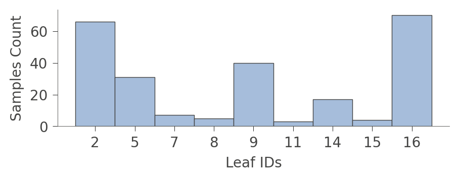
Decision trees make decisions at the leaf nodes and so it is sometimes useful to zoom in on those, particularly if the entire graph is too large to see all at once. Here is how to examine the number of training data instances that are grouped into each leaf node:
viz_cmodel.leaf_sizes(figsize=(5,1.5))
A perhaps more interesting graph is one that shows the proportion of each kind of training instance in the various leaves. The goal of training is to have leaves with a single color because it represents "pure" nodes that can predict that class with high confidence.
viz_cmodel.ctree_leaf_distributions(figsize=(5,1.5))
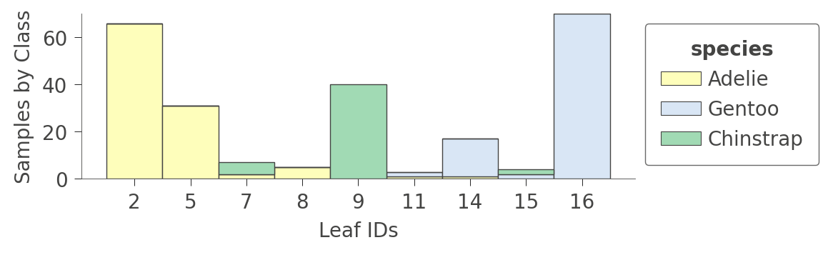
We can also zoom in on a specific leaf node to look at some stats of the various instance features. For example, leaf node 5 contains 31 instances, 24 of which have unique bill_length_mm values:
viz_cmodel.node_stats(node_id=5)
How decision trees classify an instance
Now that we've looked at the structure and contents of a decision tree, let's figure out how the classifier makes a decision for a specific instance. By passing in an instance (a feature vector) as argument x, the view() function will highlight the path from the root to the leaf pursued by the classifier to make the prediction for that instance:
x = train_ds_pd[penguin_features].iloc[20]
viz_cmodel.view(x=x, scale=.75)
/tmpfs/src/tf_docs_env/lib/python3.9/site-packages/dtreeviz/models/shadow_decision_tree.py:335: FutureWarning: Series.__getitem__ treating keys as positions is deprecated. In a future version, integer keys will always be treated as labels (consistent with DataFrame behavior). To access a value by position, use `ser.iloc[pos]`
/tmpfs/src/tf_docs_env/lib/python3.9/site-packages/dtreeviz/trees.py:1231: FutureWarning: Series.__getitem__ treating keys as positions is deprecated. In a future version, integer keys will always be treated as labels (consistent with DataFrame behavior). To access a value by position, use `ser.iloc[pos]`
/tmpfs/src/tf_docs_env/lib/python3.9/site-packages/dtreeviz/trees.py:1225: FutureWarning: Series.__getitem__ treating keys as positions is deprecated. In a future version, integer keys will always be treated as labels (consistent with DataFrame behavior). To access a value by position, use `ser.iloc[pos]`
/tmpfs/src/tf_docs_env/lib/python3.9/site-packages/dtreeviz/models/shadow_decision_tree.py:335: FutureWarning: Series.__getitem__ treating keys as positions is deprecated. In a future version, integer keys will always be treated as labels (consistent with DataFrame behavior). To access a value by position, use `ser.iloc[pos]`

The illustration highlights the tree path and the instance features that were tested (island, bill_length_mm, and flipper_length_mm).
For a very large tree, you can also ask to see just the path through the tree, and not the entire tree, by using the show_just_path parameter:
viz_cmodel.view(x=x, show_just_path=True, scale=.75)
/tmpfs/src/tf_docs_env/lib/python3.9/site-packages/dtreeviz/models/shadow_decision_tree.py:335: FutureWarning: Series.__getitem__ treating keys as positions is deprecated. In a future version, integer keys will always be treated as labels (consistent with DataFrame behavior). To access a value by position, use `ser.iloc[pos]`
/tmpfs/src/tf_docs_env/lib/python3.9/site-packages/dtreeviz/trees.py:1231: FutureWarning: Series.__getitem__ treating keys as positions is deprecated. In a future version, integer keys will always be treated as labels (consistent with DataFrame behavior). To access a value by position, use `ser.iloc[pos]`
/tmpfs/src/tf_docs_env/lib/python3.9/site-packages/dtreeviz/trees.py:1225: FutureWarning: Series.__getitem__ treating keys as positions is deprecated. In a future version, integer keys will always be treated as labels (consistent with DataFrame behavior). To access a value by position, use `ser.iloc[pos]`
/tmpfs/src/tf_docs_env/lib/python3.9/site-packages/dtreeviz/models/shadow_decision_tree.py:335: FutureWarning: Series.__getitem__ treating keys as positions is deprecated. In a future version, integer keys will always be treated as labels (consistent with DataFrame behavior). To access a value by position, use `ser.iloc[pos]`

To obtain the English interpretation for the classification of an instance, the smallest possible representation, use explain_prediction_path():
print(viz_cmodel.explain_prediction_path(x=x))
bill_length_mm < 40.6
flipper_length_mm < 206.0
island in {'Dream'}
/tmpfs/src/tf_docs_env/lib/python3.9/site-packages/dtreeviz/models/shadow_decision_tree.py:335: FutureWarning: Series.__getitem__ treating keys as positions is deprecated. In a future version, integer keys will always be treated as labels (consistent with DataFrame behavior). To access a value by position, use `ser.iloc[pos]`
/tmpfs/src/tf_docs_env/lib/python3.9/site-packages/dtreeviz/interpretation.py:54: FutureWarning: Series.__getitem__ treating keys as positions is deprecated. In a future version, integer keys will always be treated as labels (consistent with DataFrame behavior). To access a value by position, use `ser.iloc[pos]`
The model tests x's bill_length_mm, flipper_length_mm, and island features to reach the leaf, which in this case, predicts Adelie.
Feature space partitioning
So far we've looked at the structure of trees and how trees interpret instances to make decisions, but what exactly are the decision nodes doing? Decision trees partition feature space into groups of observations that share similar target values. Each leaf represents the partitioning resulting from the sequence of feature splitting performed from the root down to that leaf. For classification, the goal is to get partitions to share the same or mostly the same target class value.
If we look back at the tree structure, we see that variable flipper_length_mm is tested by three nodes in the tree. The corresponding decision node split values are 189, 206, and 210.5, which means that the decision tree is splitting flipper_length_mm into four regions, which we can illustrate using ctree_feature_space():
viz_cmodel.ctree_feature_space(features=['flipper_length_mm'], show={'splits','legend'}, figsize=(5,1.5))
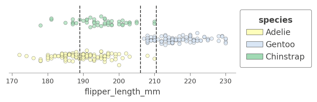
(The vertical axis is not meaningful in this single-feature case. To increase visibility, that vertical axis just separates the dots representing different target classes into different elevations with some noise added.)
The first split at 206 (tested at the root) separates the training data into an overlapping region of Adelie/Gentoo Penguins and a fairly region of Chinstrap Penguins. The subsequent split at 210.5 further isolates a region of pure Chinstrap (above 210.5 flipper length). The decision tree also splits at 189, but the resulting regions are still impure. The tree relies on splitting by other variables to separate the "confused" clumps of Adelie/Gentoo Penguins. Because we have passed in a single feature name, no splits are shown for other features.
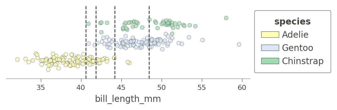
Let's look at another feature that has more splits, bill_length_mm. There are four nodes in the decision tree that test that feature and so we get a feature space split into five regions. Notice how the model can split off a pure region of Adelie by testing for bill_length_mm less than 40:
viz_cmodel.ctree_feature_space(features=['bill_length_mm'], show={'splits','legend'},
                               figsize=(5,1.5))
We can also examine the how the tree partitions feature space for two features at once, such as flipper_length_mm and bill_length_mm:
viz_cmodel.ctree_feature_space(features=['flipper_length_mm','bill_length_mm'],
                               show={'splits','legend'}, figsize=(5,5))
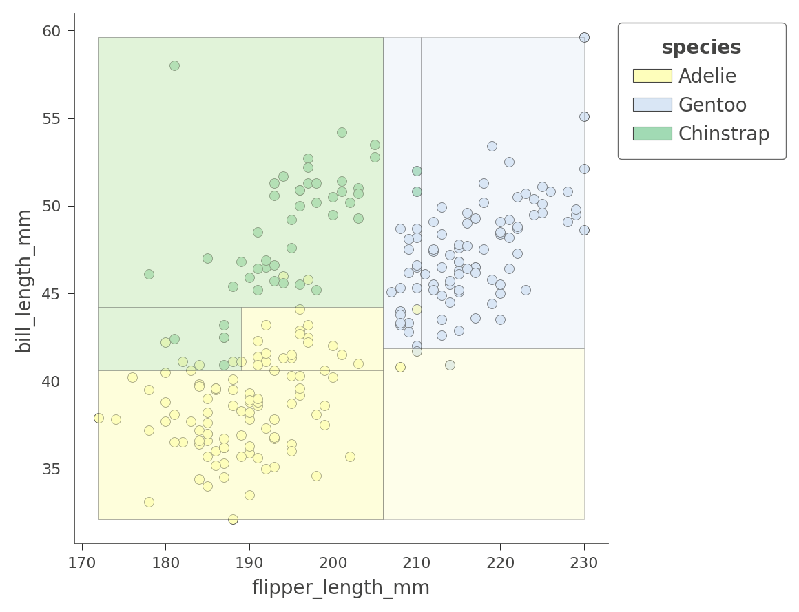
The color of the region indicates the color of the classification for test instances whose features fall in that region.
By considering two variables at once, the decision tree can create much more pure (rectangular) regions, leading to more accurate predictions. For example, the upper left region encapsulates purely Chinstrap penguins.
Depending on the variables we choose, the regions will be more or less pure. Here is another 2D feature space partition for features bill_depth_mm and bill_length_mm, where shades indicate uncertainty.
viz_cmodel.ctree_feature_space(features=['body_mass_g','bill_length_mm'],
                               show={'splits','legend'}, figsize=(5,5))
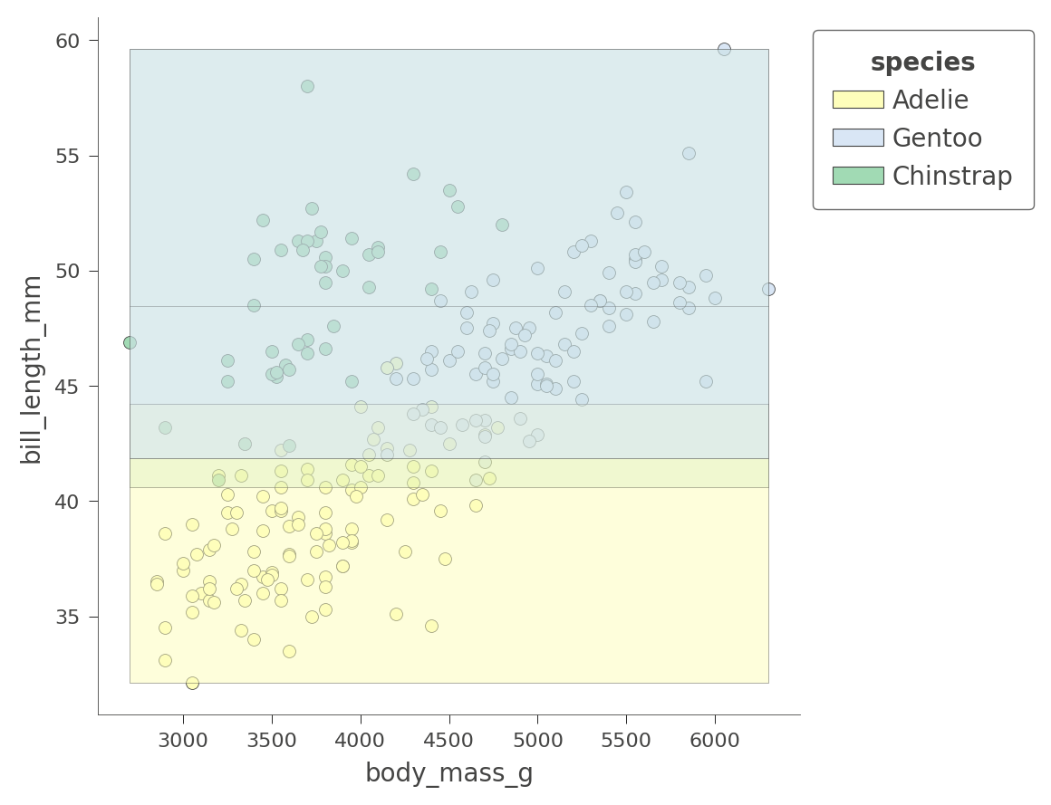
Only the Adelie region is fairly pure. The tree relies on other variables to get a better partition, as we just saw with flipper_length_mm vs bill_length_mm space.
The dtreeviz library cannot visualize more than two feature dimensions for classification at this time.
At this point, you've got a good handle on how to visualize the structure of decision trees, how trees partition feature space, and how trees classify test instances. Let's turn now to regression and see how dtreeviz visualizes regression trees.
Visualizing Regressor Trees
 Let's use the abalone dataset used in the beginner tutorial to explore the structure of regression trees. As we did for classification above, we start by loading and preparing data for training. Given 8 variables, we'd like to predict the number of rings in an abalone's shell.
Load, clean, and prep data
Using the following code snippet, we can see that the features are all numeric except for the Type (sex) variable.
# Download the dataset.
!wget -q https://storage.googleapis.com/download.tensorflow.org/data/abalone_raw.csv -O /tmp/abalone.csv

df_abalone = pd.read_csv("/tmp/abalone.csv")
df_abalone.head(3)
Fortunately, there's no missing data to deal with:
df_abalone.isna().any()
Type             False
LongestShell     False
Diameter         False
Height           False
WholeWeight      False
ShuckedWeight    False
VisceraWeight    False
ShellWeight      False
Rings            False
dtype: bool
Split train/test set and train model
abalone_label = "Rings"   # Name of the classification target label

# Split into training and test sets 70/30
df_train_abalone, df_test_abalone = split_dataset(df_abalone)
print(f"{len(df_train_abalone)} examples in training, {len(df_test_abalone)} examples for testing.")

# Convert to tensorflow data sets
train_ds = tfdf.keras.pd_dataframe_to_tf_dataset(df_train_abalone, label=abalone_label, task=tfdf.keras.Task.REGRESSION)
test_ds = tfdf.keras.pd_dataframe_to_tf_dataset(df_test_abalone, label=abalone_label, task=tfdf.keras.Task.REGRESSION)
2935 examples in training, 1242 examples for testing.
Train a random forest regressor
Now that we have training and test sets, let's train a random forest regressor. Because of the nature of the data, we need to artificially restrict the height of the tree in order to visualize it. (Restricting the tree depth is also a form of regularization to prevent overfitting.) A max depth of 5 is deep enough to be fairly accurate but small enough to visualize.
rmodel = tfdf.keras.RandomForestModel(task=tfdf.keras.Task.REGRESSION,
                                      max_depth=5,      # don't let the tree get too big
                                      random_seed=1234, # create same tree every time
                                      verbose=0)
rmodel.fit(x=train_ds)
[INFO 24-08-24 11:23:49.4411 UTC kernel.cc:1233] Loading model from path /tmpfs/tmp/tmpu2s76oqn/model/ with prefix 571755d398de4f74
[INFO 24-08-24 11:23:49.4661 UTC decision_forest.cc:734] Model loaded with 300 root(s), 9264 node(s), and 8 input feature(s).
[INFO 24-08-24 11:23:49.4661 UTC abstract_model.cc:1344] Engine "RandomForestOptPred" built
[INFO 24-08-24 11:23:49.4661 UTC kernel.cc:1061] Use fast generic engine
<tf_keras.src.callbacks.History at 0x7f676c7e2af0>
Let's check the accuracy of the model using MAE and MSE. The range of Rings is 1-27, so an MAE of 1.66 on the test set is not great but it's OK for our demonstration purposes.
# Evaluate the model on the test dataset.
rmodel.compile(metrics=["mae","mse"])
evaluation = rmodel.evaluate(test_ds, return_dict=True, verbose=0)

print(f"MSE: {evaluation['mse']}")
print(f"MAE: {evaluation['mae']}")
print(f"RMSE: {math.sqrt(evaluation['mse'])}")
MSE: 5.4397759437561035
MAE: 1.6559592485427856
RMSE: 2.3323327257825164
Display decision tree
To use dtreeviz, we need to bundle up the model and the training data. We also have to choose a particular tree from the random forest to display; let's choose tree 3 as we did for classification.
abalone_features = [f.name for f in rmodel.make_inspector().features()]
viz_rmodel = dtreeviz.model(rmodel, tree_index=3,
                           X_train=df_train_abalone[abalone_features],
                           y_train=df_train_abalone[abalone_label],
                           feature_names=abalone_features,
                           target_name='Rings')
Function view() displays the structure of the tree, but now the decision nodes are scatterplots not stacked bar charts. Each decision node shows a marginal plot of the indicated variable versus the target (Rings):
viz_rmodel.view(scale=1.2)

As with classification, regression proceeds from the root of the tree towards a specific leaf, which ultimately makes the prediction for a specific test instance. The nodes on the path to the leaf test numeric or categorical variables, directing the regressor into a specific region of feature space that (hopefully) has very similar target values.
The leaves are strip plots that show the target variable Rings values for all instances in the leaf. The horizontal parameter is not meaningful and is just a bit of noise to separate the dots so we can see where the density lies. Consider the lower left leaf with n=10, Rings=3.30. That indicates that the average Rings value for the 10 instances in that leaf is 3.30, which is then the prediction from the decision tree for any test instance that reaches that leaf.
Let's zoom in on the root of the tree to see how the regressor splits on variable ShellWeight:
viz_rmodel.view(depth_range_to_display=[0,0], scale=2)

For a test instance with ShellWeight<0.164, the regressor proceeds down the left child of the root; otherwise it proceeds down the right child. The horizontal dashed lines indicate the average Rings value associated with instances whose ShellWeight is above or below 0.164.
Decision nodes for categorical variables, on the other hand, test subsets of categories since categories are unordered. In the fourth level of the tree, there are two decision nodes that test categorical variable Type:
viz_rmodel.view(depth_range_to_display=[3,3], scale=1.5)

Regressor nodes that test categoricals use color to indicate subsets. For example, the decision node on the left at the fourth level directs the regressor to descend to the left if the test instance it has Type=I or Type=F; otherwise the regressor descends to the right. The yellow and blue colors indicate the two categorical value subsets associated with left and right branches. The horizontal dashed lines indicate the average Rings target value for instances with the associated categorical value(s).
To display large trees, you can use the orientation parameter to get a left to right version of the tree, although it is fairly tall so using scale to shrink it is a good idea. Using a screen zoom-in feature on your machine, you can zoom in on areas of interest.
viz_rmodel.view(orientation='LR', scale=.5)

We can save space with the non-fancy plot. It still shows the decision node split variables and split points; it's just not as pretty.
viz_rmodel.view(fancy=False, scale=.75)

Examining leaf stats
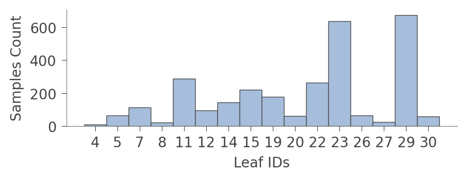
When graphs get very large, it's sometimes better to focus on the leaves. Function leaf_sizes() indicates the number of instances found in each leaf:
viz_rmodel.leaf_sizes(figsize=(5,1.5))
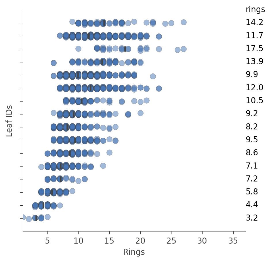
We can also look at the distribution of instances in the leaves (Rings values). The vertical axis has a "row" for each leaf and the horizontal axis shows the distribution of Rings values for instances in each leaf. The column on the right shows the average target value for each leaf.
viz_rmodel.rtree_leaf_distributions(figsize=(5,5))
Alternatively, we can get information on the features of the instances in a particular node. For example, here's how to get information on features in leaf id 29, the leaf with the most instances:
viz_rmodel.node_stats(node_id=29)
How decision trees predict a value for an instance
To make a prediction for a specific instance, the decision tree weaves its way from the root down to a specific leaf, according to the feature values in the test instance. The prediction of the individual tree is just the average of the Rings values from instances (from the training set) residing in that leaf. The dtreeviz library can illustrate this process if we provide a test instance via parameter x.
x = df_abalone[abalone_features].iloc[1234]
viz_rmodel.view(x=x, scale=.75)
/tmpfs/src/tf_docs_env/lib/python3.9/site-packages/dtreeviz/models/shadow_decision_tree.py:335: FutureWarning: Series.__getitem__ treating keys as positions is deprecated. In a future version, integer keys will always be treated as labels (consistent with DataFrame behavior). To access a value by position, use `ser.iloc[pos]`
/tmpfs/src/tf_docs_env/lib/python3.9/site-packages/dtreeviz/trees.py:1351: FutureWarning: Series.__getitem__ treating keys as positions is deprecated. In a future version, integer keys will always be treated as labels (consistent with DataFrame behavior). To access a value by position, use `ser.iloc[pos]`
/tmpfs/src/tf_docs_env/lib/python3.9/site-packages/dtreeviz/trees.py:1356: FutureWarning: Series.__getitem__ treating keys as positions is deprecated. In a future version, integer keys will always be treated as labels (consistent with DataFrame behavior). To access a value by position, use `ser.iloc[pos]`
/tmpfs/src/tf_docs_env/lib/python3.9/site-packages/dtreeviz/trees.py:1324: FutureWarning: Series.__getitem__ treating keys as positions is deprecated. In a future version, integer keys will always be treated as labels (consistent with DataFrame behavior). To access a value by position, use `ser.iloc[pos]`

If that visualization is too large, we can cut down the plot to just the path from the root to the leaf that is actually traversed:
viz_rmodel.view(x=x, show_just_path=True, scale=1.0)
/tmpfs/src/tf_docs_env/lib/python3.9/site-packages/dtreeviz/models/shadow_decision_tree.py:335: FutureWarning: Series.__getitem__ treating keys as positions is deprecated. In a future version, integer keys will always be treated as labels (consistent with DataFrame behavior). To access a value by position, use `ser.iloc[pos]`
/tmpfs/src/tf_docs_env/lib/python3.9/site-packages/dtreeviz/trees.py:1351: FutureWarning: Series.__getitem__ treating keys as positions is deprecated. In a future version, integer keys will always be treated as labels (consistent with DataFrame behavior). To access a value by position, use `ser.iloc[pos]`
/tmpfs/src/tf_docs_env/lib/python3.9/site-packages/dtreeviz/trees.py:1356: FutureWarning: Series.__getitem__ treating keys as positions is deprecated. In a future version, integer keys will always be treated as labels (consistent with DataFrame behavior). To access a value by position, use `ser.iloc[pos]`
/tmpfs/src/tf_docs_env/lib/python3.9/site-packages/dtreeviz/trees.py:1324: FutureWarning: Series.__getitem__ treating keys as positions is deprecated. In a future version, integer keys will always be treated as labels (consistent with DataFrame behavior). To access a value by position, use `ser.iloc[pos]`

We can make it even smaller using a horizontal orientation:
viz_rmodel.view(x=x, show_just_path=True, scale=.75, orientation="LR")
/tmpfs/src/tf_docs_env/lib/python3.9/site-packages/dtreeviz/models/shadow_decision_tree.py:335: FutureWarning: Series.__getitem__ treating keys as positions is deprecated. In a future version, integer keys will always be treated as labels (consistent with DataFrame behavior). To access a value by position, use `ser.iloc[pos]`
/tmpfs/src/tf_docs_env/lib/python3.9/site-packages/dtreeviz/trees.py:1351: FutureWarning: Series.__getitem__ treating keys as positions is deprecated. In a future version, integer keys will always be treated as labels (consistent with DataFrame behavior). To access a value by position, use `ser.iloc[pos]`
/tmpfs/src/tf_docs_env/lib/python3.9/site-packages/dtreeviz/trees.py:1356: FutureWarning: Series.__getitem__ treating keys as positions is deprecated. In a future version, integer keys will always be treated as labels (consistent with DataFrame behavior). To access a value by position, use `ser.iloc[pos]`
/tmpfs/src/tf_docs_env/lib/python3.9/site-packages/dtreeviz/trees.py:1324: FutureWarning: Series.__getitem__ treating keys as positions is deprecated. In a future version, integer keys will always be treated as labels (consistent with DataFrame behavior). To access a value by position, use `ser.iloc[pos]`

Sometimes it's easier just to get an English description of how the model tested our feature values to make a decision:
print(viz_rmodel.explain_prediction_path(x=x))
0.25 <= Diameter
ShellWeight < 0.11
Type not in {'M', 'F'}
/tmpfs/src/tf_docs_env/lib/python3.9/site-packages/dtreeviz/models/shadow_decision_tree.py:335: FutureWarning: Series.__getitem__ treating keys as positions is deprecated. In a future version, integer keys will always be treated as labels (consistent with DataFrame behavior). To access a value by position, use `ser.iloc[pos]`
/tmpfs/src/tf_docs_env/lib/python3.9/site-packages/dtreeviz/interpretation.py:54: FutureWarning: Series.__getitem__ treating keys as positions is deprecated. In a future version, integer keys will always be treated as labels (consistent with DataFrame behavior). To access a value by position, use `ser.iloc[pos]`
Feature space partitioning
Using rtree_feature_space(), we can see how the decision tree partitions a feature space via a collection of splits. For example, here is how the decision tree partitions feature ShellWeight:
viz_rmodel.rtree_feature_space(features=['ShellWeight'],
                              show={'splits'})
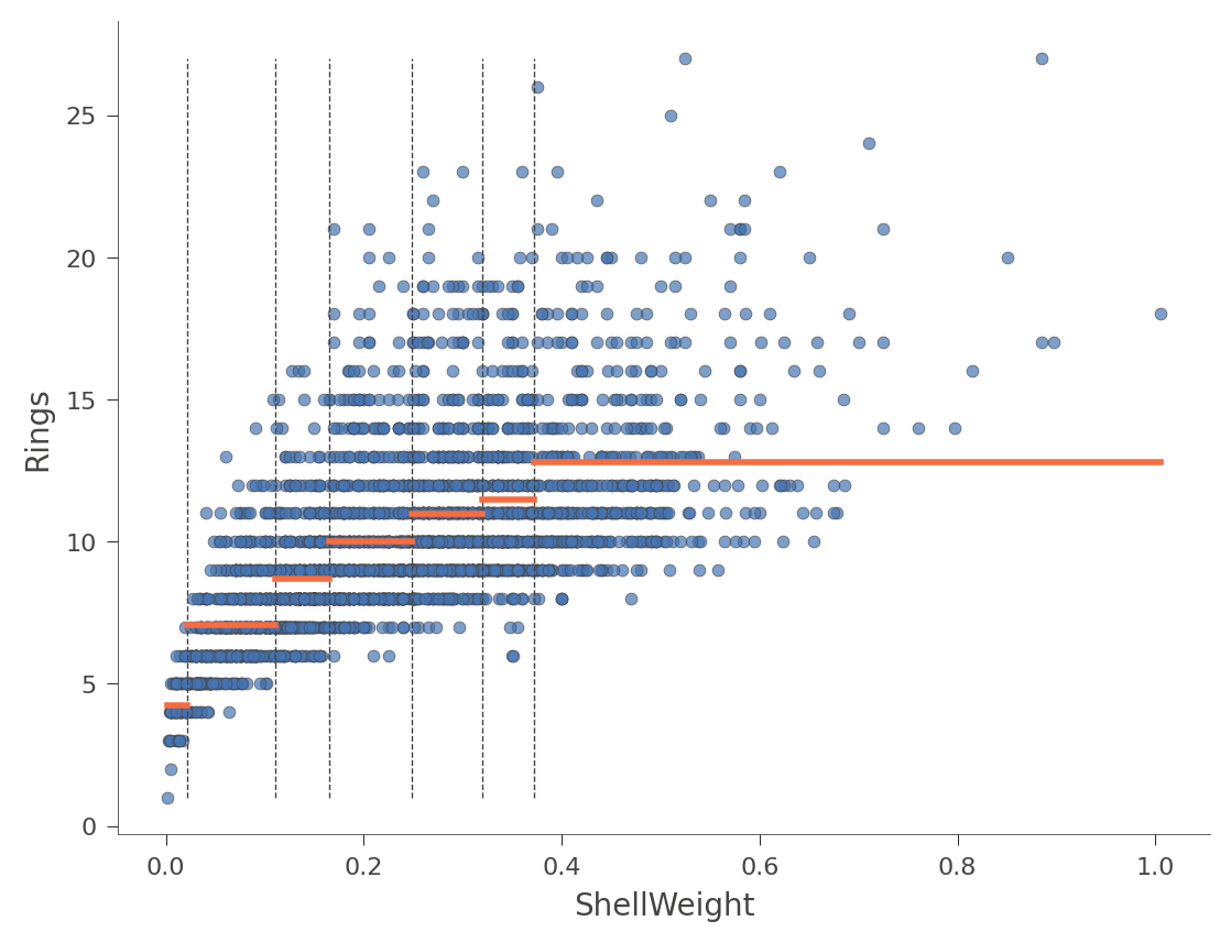
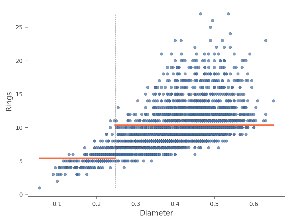
The horizontal orange bars indicate the average Rings value within each region. Here's another example using feature Diameter (with only one split in the tree):
viz_rmodel.rtree_feature_space(features=['Diameter'], show={'splits'})
We can also look at two dimensional feature space, where the Rings values vary in color from green (low) to blue (high):
viz_rmodel.rtree_feature_space(features=['ShellWeight','LongestShell'], show={'splits'})
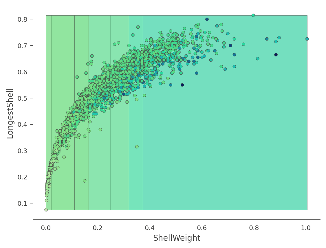
That heat map can be confusing because it's really a 2D projection of a 3D space: two features x target value. Instead, dtreeviz can show you this three-dimensional plot (from a variety of angles and elevations):
viz_rmodel.rtree_feature_space3D(features=['ShellWeight','LongestShell'],
                              show={'splits'}, elev=30, azim=140, dist=11, figsize=(9,8))
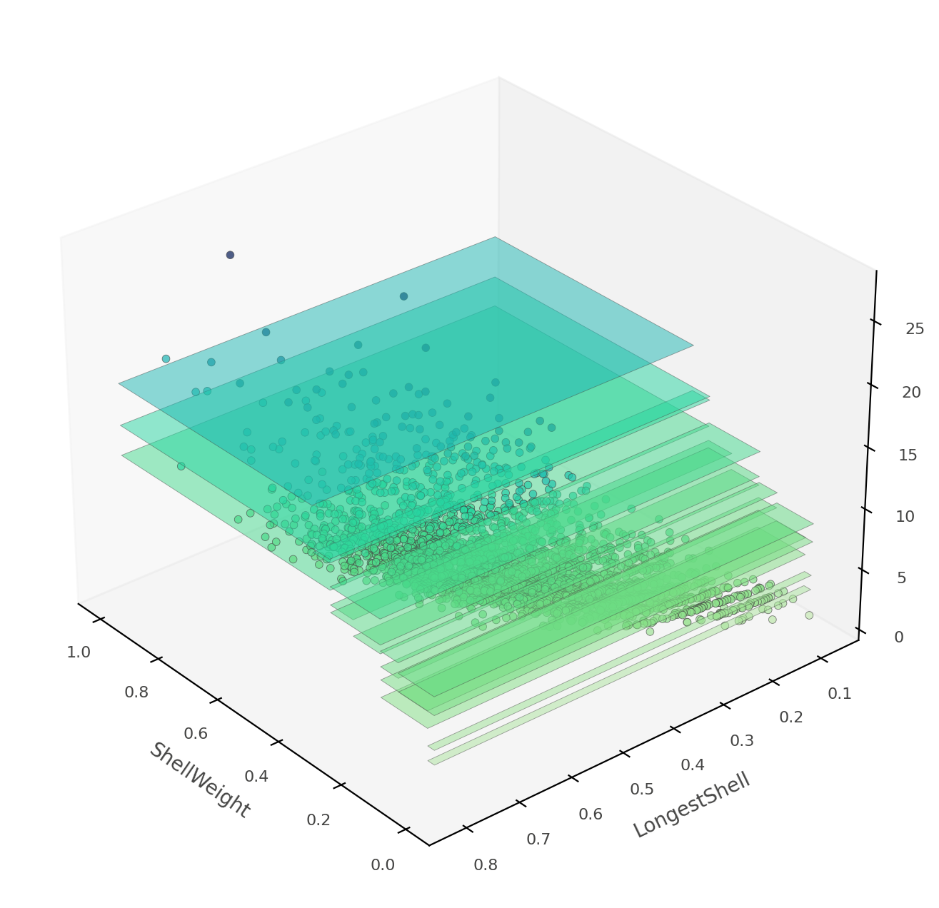
If ShellWeight and LongestShell were the only features tested by the model, there would be no overlapping vertical "plates". Each 2D region of feature space would make a unique prediction. In this tree, there are other features that differentiate between ambiguous vertical prediction regions.
At this point, you've learned how to use dtreeviz to display the structure of decision trees, plot leaf information, trace how a model interprets a specific instance, and how a model partitions future space. You're ready to visualize and interpret trees using your own data sets!
From here, you might also consider checking out these colabs: Intermediate colab or Making predictions.