
 GitHub でソースを表示 GitHub でソースを表示 |
概要
GPU と TPU は、単一のトレーニングステップを実行するために必要な時間を劇的に短縮することができます。ピークパフォーマンスの達成には、現在のステップが終了する前に、次のステップのデータを配信する有効な入力パイプラインが必要となります。柔軟で効率的な入力パイプラインの構築に役立つのが、tf.data API です。このドキュメントでは、tf.data API を使用して非常に性能の高い TensorFlow 入力パイプラインを構築する方法を説明します。
読み進める前に、「TensorFlow 入力パイプラインの構築」ガイドに目を通し、tf.data API の使用方法を学習してください。
リソース
セットアップ
import tensorflow as tf

import time
2022-12-14 20:12:40.389570: W tensorflow/compiler/xla/stream_executor/platform/default/dso_loader.cc:64] Could not load dynamic library 'libnvinfer.so.7'; dlerror: libnvinfer.so.7: cannot open shared object file: No such file or directory
2022-12-14 20:12:40.389666: W tensorflow/compiler/xla/stream_executor/platform/default/dso_loader.cc:64] Could not load dynamic library 'libnvinfer_plugin.so.7'; dlerror: libnvinfer_plugin.so.7: cannot open shared object file: No such file or directory
2022-12-14 20:12:40.389675: W tensorflow/compiler/tf2tensorrt/utils/py_utils.cc:38] TF-TRT Warning: Cannot dlopen some TensorRT libraries. If you would like to use Nvidia GPU with TensorRT, please make sure the missing libraries mentioned above are installed properly.
このガイドでは、データセットをイテレートし、パフォーマンスを測定します。次のようなさまざまな要因の影響により、再現可能なパフォーマンスベンチマークを作成することが困難となる場合があります。
- 現在の CPU 負荷
- ネットワークトラフィック
- キャッシュなどの複雑なメガニズム
再現可能なベンチマークを提供するために、人工的な例を構築します。
データセット
まずは、ArtificialDataset という、tf.data.Dataset から継承するクラスを定義します。このデータセットは次のことを行います。
num_samplesサンプルを生成する(デフォルトは 3)- ファイルを開くアクションをシミュレーションするために、最初のアイテムの前にしばらくスリープする
- ファイルからデータを読み込む操作をシミュレーションするために、各アイテムを生成する前にしばらくスリープする
class ArtificialDataset(tf.data.Dataset):
    def _generator(num_samples):
        # Opening the file
        time.sleep(0.03)

        for sample_idx in range(num_samples):
            # Reading data (line, record) from the file
            time.sleep(0.015)

            yield (sample_idx,)

    def __new__(cls, num_samples=3):
        return tf.data.Dataset.from_generator(
            cls._generator,
            output_signature = tf.TensorSpec(shape = (1,), dtype = tf.int64),
            args=(num_samples,)
        )
このデータセットは tf.data.Dataset.range に似ており、各サンプルの開始とサンプル間に一定の遅延を追加します。
トレーニングループ
次に、データセットのイテレートにどれくらいの時間がかかるかを測定するダミーのトレーニングループを記述します。トレーニング時間がシミュレーションされます。
def benchmark(dataset, num_epochs=2):
    start_time = time.perf_counter()
    for epoch_num in range(num_epochs):
        for sample in dataset:
            # Performing a training step
            time.sleep(0.01)
    print("Execution time:", time.perf_counter() - start_time)
パフォーマンスの最適化
パフォーマンスをどのように最適化できるかを示すために、ArtificialDataset のパフォーマンスを改善します。
単純なアプローチ
コツを使わずに、単純なパイプラインから始め、ありのままのデータセットをイテレートします。
benchmark(ArtificialDataset())
Execution time: 0.2333629889999429
内部的には、次のように実行時間が使われています。

プロットに、トレーニングステップの実行には、次のアクションが伴うことが示されます。
- ファイルが開いていない場合は、ファイルを開く
- ファイルからデータをフェッチする
- トレーニングにデータを使用する
ところが、このように単純な同期実装では、パイプラインがデータをフェッチしている間、モデルはアイドル状態となります。その反対に、モデルがトレーニング中である場合、入力パイプラインがアイドル状態となります。したがって、トレーニングのステップ時間は、開いて、読み取り、トレーニングする時間の和であるということになります。
次のセクションでは、この入力パイプラインに基づいて構築し、性能の高い TensorFlow 入力パイプライン設計のベストプラクティスを説明します。
プリフェッチ
プリフェッチは、トレーニングステップの事前処理とモデルの実行に重なって行われます。モデルがトレーニングステップ s を実行する間、入力パイプラインはステップ s+1 のデータを読み取っています。そうすることで、ステップ時間をトレーニングと、データの抽出にかかる時間の最大時間(和とは反対に)に減少させることができます。
tf.data API は、tf.data.Dataset.prefetch 変換を提供します。データが生成された時間をデータが消費された時間から切り離すために使用できます。具体的には、この変換は、バックグラウンドのスレッドと内部バッファを使用して、要求される前に入力データセットから要素をプリフェッチします。プリフェッチする要素の数は、単一のトレーニングステップによって消費されるバッチの数と同等(またはそれ以上)である必要があります。この値を手動で調整するか、tf.data.AUTOTUNE に設定することができますが、後者の場合、tf.data ランタイムによって、ランタイム時に動的に値が調整されます。
プリフェッチ変換は、「プロデューサ」の作業と「コンシューマ」の作業をオーバーラップする機会があればいつでもオーバーラップさせることに注意してください。
benchmark(
    ArtificialDataset()
    .prefetch(tf.data.AUTOTUNE)
)
Execution time: 0.23058086499997898

次に、サンプル 0 でトレーニングセットアップが実行している間、入力パイプラインはサンプル 1 のデータを読み取っているのがわかります。
データ抽出の並列化
実世界の状況では、入力データはリモート(Google Cloud Storage や HDFS など)に保管されていることがあります。ローカルとリモートのストレージには、次のような違いがあるため、ローカルでのデータ読み取りに適したデータセットパイプラインは、リモートで読み取られる際にボトルネックとなる可能性があります。
- 最初のバイトまでの時間: リモートストレージからファイルの最初のバイトを読み取る場合、ロカールストレージからよりもずっと長い時間がかかります。
- 読み取りのスループット: リモートストレージの総帯域幅は一般的に大きいため、単一のファイルの読み取りには、この帯域幅のほんのわずかしか使用されません。
さらに、生のバイトがメモリに読み込まれると、データのデシリアライズや復号化する必要も出てくるため(protobuf など)、さらに計算が必要となります。このオーバーヘッドは、データの格納場所がローカルであるかリモートであるかに関係なく存在しますが、データのプリフェッチが効果的に行われない場合、リモートの場合に大きくなることがあります。
データ抽出にまつわるさまざまなオーバーヘッドの影響を緩和するために、tf.data.Dataset.interleave 変換を使用して、データの読み込みステップをほかのデータセットのコンテンツ(データファイルリーダーなど)とインターリーブしながら並列化することができます。オーバーラップするデータセットの数は、cycle_length 引数で指定し、並列化のレベルは num_parallel_calls 引数で指定することができます。prefetch 変換と同様に、interleave 変換も tf.data.AUTOTUNE をサポートしているため、どのレベルの並列化を使用するかという判断は tf.data ランタイムに委ねられます。
順次インターリーブ
tf.data.Dataset.interleave 変換のデフォルトの引数によって、2 つのデータセットからの単一のサンプルが順次、インターリブされます。
benchmark(
    tf.data.Dataset.range(2)
    .interleave(lambda _: ArtificialDataset())
)
WARNING:tensorflow:From /tmpfs/src/tf_docs_env/lib/python3.9/site-packages/tensorflow/python/autograph/pyct/static_analysis/liveness.py:83: Analyzer.lamba_check (from tensorflow.python.autograph.pyct.static_analysis.liveness) is deprecated and will be removed after 2023-09-23.
Instructions for updating:
Lambda fuctions will be no more assumed to be used in the statement where they are used, or at least in the same block. https://github.com/tensorflow/tensorflow/issues/56089
Execution time: 0.4100713720000613

この図は、interleave 変換の動作を示しており、利用できる 2 つのデータセットからサンプルが交互にフェッチされています。ただし、ここでは、パフォーマンスの改善は認められません。
並列インターリーブ
では、interleave 変換の num_parallel_calls 引数を使用してみましょう。これは、複数のデータセットを並列して読み込むため、ファイルが開かれるまでの待機時間が短縮されます。
benchmark(
    tf.data.Dataset.range(2)
    .interleave(
        lambda _: ArtificialDataset(),
        num_parallel_calls=tf.data.AUTOTUNE
    )
)
Execution time: 0.31014879800000017

今度は、データ実行時間のプロットからわかるように、2 つのデータセットの読み取りが並列化され、総合的なデータ処理時間が短縮されています。
データ変換の並列化
データを準備する際、入力要素を事前処理する必要がある場合があります。この目的により、tf.data API は、ユーザー定義関数を入力データセットの各要素に適用する tf.data.Dataset.map 変換を提供しています。入力要素は互いに独立しているため、複数の CPU コアで事前処理を並列化することができます。これを行うために、prefetch と interleave 変換と同様に、map 変換でも num_parallel_calls 引数によって並列化のレベルを指定することができます。
num_parallel_calls 引数に最適な値を選択するには、ハードウェア、トレーニングデータの特性(サイズや形状など)、マップ関数のコスト、および CPU で同時に発生しているほかの処理を考慮する必要があります。簡単な調べ方は、利用可能な CPU コアの数を使用することですが、prefetch と interleave 変換に関して言えば、map 変換は tf.data.AUTOTUNE をサポートしているため、どのレベルの並列化を使用するかという判断は tf.data ランタイムに委ねられています。
def mapped_function(s):
    # Do some hard pre-processing
    tf.py_function(lambda: time.sleep(0.03), [], ())
    return s
順次マッピング
基本の例として、並列化を使用せずに map 変換を使用することから始めてみましょう。
benchmark(
    ArtificialDataset()
    .map(mapped_function)
)
Execution time: 0.4240529329999845
単純なアプローチについて言えば、ステップを開いて読み取り、事前処理(マッピング)を行ってトレーニングする時間が、単一のイテレーションの総和となります。
並列マッピング
では、同じ事前処理関数を使用して、複数のサンプルで並列に適用してみましょう。
benchmark(
    ArtificialDataset()
    .map(
        mapped_function,
        num_parallel_calls=tf.data.AUTOTUNE
    )
)
Execution time: 0.30054549199996927

データプロットが示すように、事前処理ステップがオーバーラップしたことで、単一のイテレーションにかかる総合時間が短縮されたことがわかります。
キャッシング
tf.data.Dataset.cache 変換は、メモリまたはローカルストレージのいずれかに、データセットをキャッシュすることができるため、各エポック中に一部の操作(ファイルを開いてデータを読み取るなど)が実行されなくなります。
benchmark(
    ArtificialDataset()
    .map(  # Apply time consuming operations before cache
        mapped_function
    ).cache(
    ),
    5
)
Execution time: 0.3522251550000419
ここでは、データ実行時間プロットは、データセットをキャッシュすると、cache 1 の前の変換(ファイルを開いてデータを読み取るなど)は、最初のエポックにのみ実行されることを示しています。次のエポックは、cache 変換によってキャッシュされたデータを再利用するようになります。
map 変換に渡されるユーザー定義関数が高くつく場合は、map 変換の後に cache 変換を適用することができますが、これは、キャッシュされるデータセットがメモリやローカルストレージにまだ格納できる場合に限ります。ユーザー定義関数によってデータセットを格納するために必要な容量がキャッシュのキャパシティを超えるほど増加する場合は、cache 変換の後に適用するようにするか、トレーニングジョブの前にデータを事前処理することでリソースの使用率を抑えることを検討してください。
マッピングのベクトル化
map 変換に渡されたユーザー定義関数を呼び出すと、ユーザー定義関数のスケジューリングと実行に関連するオーバーヘッドが生じます。ユーザー定義関数をベクトル化し(1 つの入力バッチでまとめて操作させる)、map 変換の前に batch 変換を適用してください。
これに適した実践を示すには、artificial データセットは適していません。スケジューリングの遅延は約 10 マイクロ秒(10e-6 秒)であり、ArtificialDataset で使用される数十ミリ秒よりはるかに短いため、その影響がわかりづらいからです。
この例では、基本の tf.data.Dataset.range 関数を使用し、トレーニングループを最も単純な形態まで単純化します。
fast_dataset = tf.data.Dataset.range(10000)

def fast_benchmark(dataset, num_epochs=2):
    start_time = time.perf_counter()
    for _ in tf.data.Dataset.range(num_epochs):
        for _ in dataset:
            pass
    tf.print("Execution time:", time.perf_counter() - start_time)

def increment(x):
    return x+1
スカラマッピング
fast_benchmark(
    fast_dataset
    # Apply function one item at a time
    .map(increment)
    # Batch
    .batch(256)
)
Execution time: 0.24833615400007147

上の図は、何が起きているかを示しています(より少ないサンプル数で)。マッピングされた関数が各サンプルに適用されているのがわかります。この関数は非常に高速ですが、時間パフォーマンスに影響するオーバーヘッドがあります。
ベクトル化されたマッピング
fast_benchmark(
    fast_dataset
    .batch(256)
    # Apply function on a batch of items
    # The tf.Tensor.__add__ method already handle batches
    .map(increment)
)
Execution time: 0.03465816100003849

今度は、マッピングされた関数は一度だけ呼び出され、サンプルのバッチに適用されています。データ実行時間のプロットが示すように、関数の実行にかかる時間は長くなりますが、オーバーヘッドの発生は一度だけであり、総合的な時間パフォーマンスが改善されています。
メモリフットプリントの縮小
interleave、prefetch、および shuffle といった多数の変換は、要素の内部バッファにとどまります。map 変換に渡されるユーザー定義関数が要素のサイズを変更すると、map 変換の順序付けと、要素をバッファリングする変換によって、メモリ使用率に影響が及びます。通常、パフォーマンスの目的でほかの順序が求められない限り、メモリフットプリントがより少なくなる順序を選択してください。
部分計算のキャッシング
メモリに入りきれないほどのデータに増加する場合を除き、map 変換の後にデータセットをキャッシュすることが推奨されます。マッピングされた関数を、時間を消費するものとメモリを消費するものの 2 つに分割できれば、トレードオフを解消することができます。この場合、次のように変換をつなぐことができます。
dataset.map(time_consuming_mapping).cache().map(memory_consuming_mapping)
こうすることで、時間を消費する部分は最初のエポック中にのみ実行されるようになるため、キャッシュスペースを使いすぎなくて済みます。
ベストプラクティスのまとめ
性能の高い TensorFlow 入力パイプライン設計のベストプラクティスをまとめてましょう。
prefetch変換を使用して、プロデューサとコンシューマの作業をオーバーラップさせる。interleave変換を使用して、データの読み取り変換を並列化する。num_parallel_calls引数を設定して、map変換を並列化する。cache変換を使用して、最初のエポック中にデータをメモリにキャッシュする。map変換に渡されるユーザー定義関数をベクトル化する。interleave、prefetch、およびshuffle変換を適用する際に、メモリ使用率を低減する。
数値の再現
注意: これ以降のノートブックでは、上記の数値を再現する方法を説明しています。このコードを自由に調整してかまいませんが、このチュートリアルの要点ではないことに留意してください。
tf.data.Dataset API の理解をさらに深めるには、独自のパイプラインで調整を試すのがよいでしょう。以下は、このガイドの画像を作成するために使用したコードです。次のような一般的な課題の回避策を示しているため、出発点にはご利用ください。
- 実行時間の再現可能性
- マッピングされた関数の Eager execution
interleave変換のコーラブル
import itertools
from collections import defaultdict

import numpy as np
import matplotlib as mpl
import matplotlib.pyplot as plt
データセット
ArtificialDataset と同様に、各ステップにかかった時間を返すデータセットを構築できます。
class TimeMeasuredDataset(tf.data.Dataset):
    # OUTPUT: (steps, timings, counters)
    OUTPUT_TYPES = (tf.dtypes.string, tf.dtypes.float32, tf.dtypes.int32)
    OUTPUT_SHAPES = ((2, 1), (2, 2), (2, 3))

    _INSTANCES_COUNTER = itertools.count()  # Number of datasets generated
    _EPOCHS_COUNTER = defaultdict(itertools.count)  # Number of epochs done for each dataset

    def _generator(instance_idx, num_samples):
        epoch_idx = next(TimeMeasuredDataset._EPOCHS_COUNTER[instance_idx])

        # Opening the file
        open_enter = time.perf_counter()
        time.sleep(0.03)
        open_elapsed = time.perf_counter() - open_enter

        for sample_idx in range(num_samples):
            # Reading data (line, record) from the file
            read_enter = time.perf_counter()
            time.sleep(0.015)
            read_elapsed = time.perf_counter() - read_enter

            yield (
                [("Open",), ("Read",)],
                [(open_enter, open_elapsed), (read_enter, read_elapsed)],
                [(instance_idx, epoch_idx, -1), (instance_idx, epoch_idx, sample_idx)]
            )
            open_enter, open_elapsed = -1., -1.  # Negative values will be filtered


    def __new__(cls, num_samples=3):
        return tf.data.Dataset.from_generator(
            cls._generator,
            output_types=cls.OUTPUT_TYPES,
            output_shapes=cls.OUTPUT_SHAPES,
            args=(next(cls._INSTANCES_COUNTER), num_samples)
        )
このデータセットは、形状 [[2, 1], [2, 2], [2, 3]] と型 [tf.dtypes.string, tf.dtypes.float32, tf.dtypes.int32] のサンプルを提供します。各サンプルは、次のとおりです。
(
  [("Open"), ("Read")],
  [(t0, d), (t0, d)],
  [(i, e, -1), (i, e, s)]
)
次のように解釈してください。
OpenとReadはステップ識別子t0は、対応するステップが開始した時間のタイムスタンプdは、対応するステップにかかった時間iはインスタンスのインデックスeはエポックのインデックス(データセットがイテレートした回数)sはサンプルのインデックス
イテレーションループ
すべてのタイミングを収集できるように、イテレーションループを多少複雑化するとよいでしょう。これは、上記に説明したサンプルを生成するデータセットでのみ機能します。
def timelined_benchmark(dataset, num_epochs=2):
    # Initialize accumulators
    steps_acc = tf.zeros([0, 1], dtype=tf.dtypes.string)
    times_acc = tf.zeros([0, 2], dtype=tf.dtypes.float32)
    values_acc = tf.zeros([0, 3], dtype=tf.dtypes.int32)

    start_time = time.perf_counter()
    for epoch_num in range(num_epochs):
        epoch_enter = time.perf_counter()
        for (steps, times, values) in dataset:
            # Record dataset preparation informations
            steps_acc = tf.concat((steps_acc, steps), axis=0)
            times_acc = tf.concat((times_acc, times), axis=0)
            values_acc = tf.concat((values_acc, values), axis=0)

            # Simulate training time
            train_enter = time.perf_counter()
            time.sleep(0.01)
            train_elapsed = time.perf_counter() - train_enter

            # Record training informations
            steps_acc = tf.concat((steps_acc, [["Train"]]), axis=0)
            times_acc = tf.concat((times_acc, [(train_enter, train_elapsed)]), axis=0)
            values_acc = tf.concat((values_acc, [values[-1]]), axis=0)

        epoch_elapsed = time.perf_counter() - epoch_enter
        # Record epoch informations
        steps_acc = tf.concat((steps_acc, [["Epoch"]]), axis=0)
        times_acc = tf.concat((times_acc, [(epoch_enter, epoch_elapsed)]), axis=0)
        values_acc = tf.concat((values_acc, [[-1, epoch_num, -1]]), axis=0)
        time.sleep(0.001)

    tf.print("Execution time:", time.perf_counter() - start_time)
    return {"steps": steps_acc, "times": times_acc, "values": values_acc}
作図方法
最後に、timelined_benchmark 関数によって返された値でタイムラインを作図できる関数を定義します。
def draw_timeline(timeline, title, width=0.5, annotate=False, save=False):
    # Remove invalid entries (negative times, or empty steps) from the timelines
    invalid_mask = np.logical_and(timeline['times'] > 0, timeline['steps'] != b'')[:,0]
    steps = timeline['steps'][invalid_mask].numpy()
    times = timeline['times'][invalid_mask].numpy()
    values = timeline['values'][invalid_mask].numpy()

    # Get a set of different steps, ordered by the first time they are encountered
    step_ids, indices = np.stack(np.unique(steps, return_index=True))
    step_ids = step_ids[np.argsort(indices)]

    # Shift the starting time to 0 and compute the maximal time value
    min_time = times[:,0].min()
    times[:,0] = (times[:,0] - min_time)
    end = max(width, (times[:,0]+times[:,1]).max() + 0.01)

    cmap = mpl.cm.get_cmap("plasma")
    plt.close()
    fig, axs = plt.subplots(len(step_ids), sharex=True, gridspec_kw={'hspace': 0})
    fig.suptitle(title)
    fig.set_size_inches(17.0, len(step_ids))
    plt.xlim(-0.01, end)

    for i, step in enumerate(step_ids):
        step_name = step.decode()
        ax = axs[i]
        ax.set_ylabel(step_name)
        ax.set_ylim(0, 1)
        ax.set_yticks([])
        ax.set_xlabel("time (s)")
        ax.set_xticklabels([])
        ax.grid(which="both", axis="x", color="k", linestyle=":")

        # Get timings and annotation for the given step
        entries_mask = np.squeeze(steps==step)
        serie = np.unique(times[entries_mask], axis=0)
        annotations = values[entries_mask]

        ax.broken_barh(serie, (0, 1), color=cmap(i / len(step_ids)), linewidth=1, alpha=0.66)
        if annotate:
            for j, (start, width) in enumerate(serie):
                annotation = "\n".join([f"{l}: {v}" for l,v in zip(("i", "e", "s"), annotations[j])])
                ax.text(start + 0.001 + (0.001 * (j % 2)), 0.55 - (0.1 * (j % 2)), annotation,
                        horizontalalignment='left', verticalalignment='center')
    if save:
        plt.savefig(title.lower().translate(str.maketrans(" ", "_")) + ".svg")
マッピングされた関数にラッパーを使用
マッピングされた関数を Eager コンテキストで実行するには、それらをtf.py_function 呼び出し内にラップする必要があります。
def map_decorator(func):
    def wrapper(steps, times, values):
        # Use a tf.py_function to prevent auto-graph from compiling the method
        return tf.py_function(
            func,
            inp=(steps, times, values),
            Tout=(steps.dtype, times.dtype, values.dtype)
        )
    return wrapper
パイプラインの比較
_batch_map_num_items = 50

def dataset_generator_fun(*args):
    return TimeMeasuredDataset(num_samples=_batch_map_num_items)
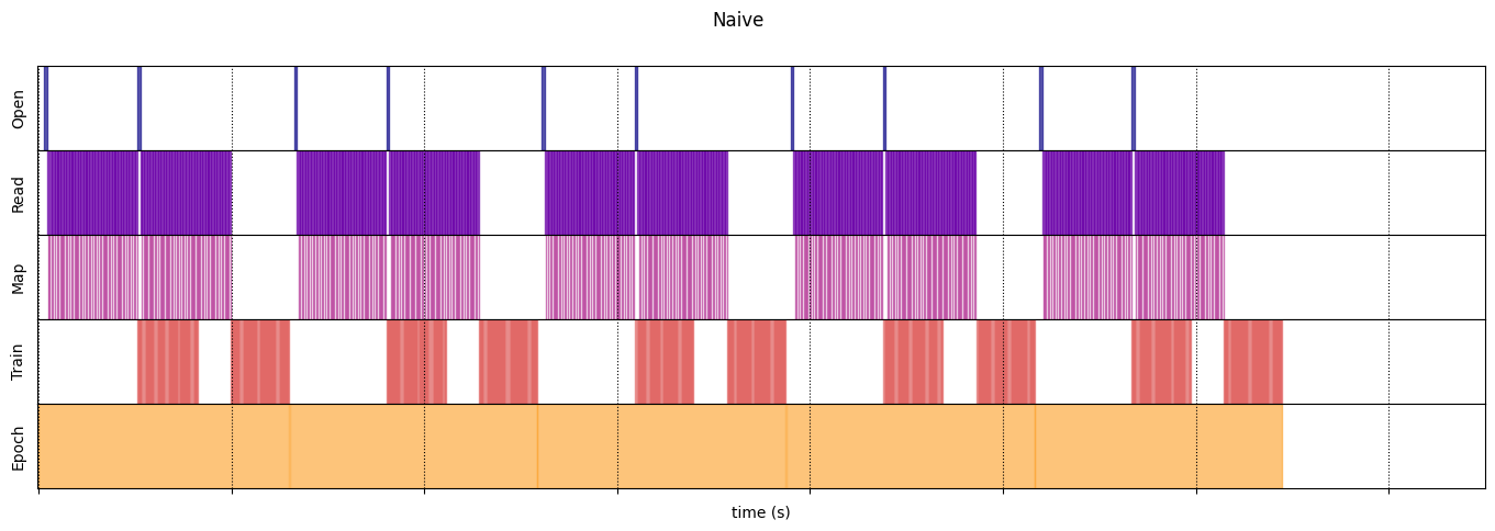
単純
@map_decorator
def naive_map(steps, times, values):
    map_enter = time.perf_counter()
    time.sleep(0.001)  # Time consuming step
    time.sleep(0.0001)  # Memory consuming step
    map_elapsed = time.perf_counter() - map_enter

    return (
        tf.concat((steps, [["Map"]]), axis=0),
        tf.concat((times, [[map_enter, map_elapsed]]), axis=0),
        tf.concat((values, [values[-1]]), axis=0)
    )

naive_timeline = timelined_benchmark(
    tf.data.Dataset.range(2)
    .flat_map(dataset_generator_fun)
    .map(naive_map)
    .batch(_batch_map_num_items, drop_remainder=True)
    .unbatch(),
    5
)
WARNING:tensorflow:From /tmpfs/tmp/ipykernel_23190/64197174.py:32: calling DatasetV2.from_generator (from tensorflow.python.data.ops.dataset_ops) with output_types is deprecated and will be removed in a future version.
Instructions for updating:
Use output_signature instead
WARNING:tensorflow:From /tmpfs/tmp/ipykernel_23190/64197174.py:32: calling DatasetV2.from_generator (from tensorflow.python.data.ops.dataset_ops) with output_shapes is deprecated and will be removed in a future version.
Instructions for updating:
Use output_signature instead
Execution time: 12.898758070999975
最適化
@map_decorator
def time_consuming_map(steps, times, values):
    map_enter = time.perf_counter()
    time.sleep(0.001 * values.shape[0])  # Time consuming step
    map_elapsed = time.perf_counter() - map_enter

    return (
        tf.concat((steps, tf.tile([[["1st map"]]], [steps.shape[0], 1, 1])), axis=1),
        tf.concat((times, tf.tile([[[map_enter, map_elapsed]]], [times.shape[0], 1, 1])), axis=1),
        tf.concat((values, tf.tile([[values[:][-1][0]]], [values.shape[0], 1, 1])), axis=1)
    )


@map_decorator
def memory_consuming_map(steps, times, values):
    map_enter = time.perf_counter()
    time.sleep(0.0001 * values.shape[0])  # Memory consuming step
    map_elapsed = time.perf_counter() - map_enter

    # Use tf.tile to handle batch dimension
    return (
        tf.concat((steps, tf.tile([[["2nd map"]]], [steps.shape[0], 1, 1])), axis=1),
        tf.concat((times, tf.tile([[[map_enter, map_elapsed]]], [times.shape[0], 1, 1])), axis=1),
        tf.concat((values, tf.tile([[values[:][-1][0]]], [values.shape[0], 1, 1])), axis=1)
    )


optimized_timeline = timelined_benchmark(
    tf.data.Dataset.range(2)
    .interleave(  # Parallelize data reading
        dataset_generator_fun,
        num_parallel_calls=tf.data.AUTOTUNE
    )
    .batch(  # Vectorize your mapped function
        _batch_map_num_items,
        drop_remainder=True)
    .map(  # Parallelize map transformation
        time_consuming_map,
        num_parallel_calls=tf.data.AUTOTUNE
    )
    .cache()  # Cache data
    .map(  # Reduce memory usage
        memory_consuming_map,
        num_parallel_calls=tf.data.AUTOTUNE
    )
    .prefetch(  # Overlap producer and consumer works
        tf.data.AUTOTUNE
    )
    .unbatch(),
    5
)
Execution time: 6.640523429000041
draw_timeline(naive_timeline, "Naive", 15)
draw_timeline(optimized_timeline, "Optimized", 15)
