|
|
|
 View source on GitHub View source on GitHub
|
|
Overview
One of the biggest challanges in Automatic Speech Recognition is the preparation and augmentation of audio data. Audio data analysis could be in time or frequency domain, which adds additional complex compared with other data sources such as images.
As a part of the TensorFlow ecosystem, tensorflow-io package provides quite a few useful audio-related APIs that helps easing the preparation and augmentation of audio data.
Setup
Install required Packages, and restart runtime
pip install tensorflow-ioUsage
Read an Audio File
In TensorFlow IO, class tfio.audio.AudioIOTensor allows you to read an audio file into a lazy-loaded IOTensor:
import tensorflow as tf
import tensorflow_io as tfio

audio = tfio.audio.AudioIOTensor('gs://cloud-samples-tests/speech/brooklyn.flac')

print(audio)
<AudioIOTensor: shape=[28979 1], dtype=<dtype: 'int16'>, rate=16000>
In the above example, the Flac file brooklyn.flac is from a publicly accessible audio clip in google cloud.
The GCS address gs://cloud-samples-tests/speech/brooklyn.flac are used directly because GCS is a supported file system in TensorFlow. In addition to Flac format, WAV, Ogg, MP3, and MP4A are also supported by AudioIOTensor with automatic file format detection.
AudioIOTensor is lazy-loaded so only shape, dtype, and sample rate are shown initially. The shape of the AudioIOTensor is represented as [samples, channels], which means the audio clip you loaded is mono channel with 28979 samples in int16.
The content of the audio clip will only be read as needed, either by converting AudioIOTensor to Tensor through to_tensor(), or though slicing. Slicing is especially useful when only a small portion of a large audio clip is needed:
audio_slice = audio[100:]

# remove last dimension
audio_tensor = tf.squeeze(audio_slice, axis=[-1])

print(audio_tensor)
tf.Tensor([16 39 66 ... 56 81 83], shape=(28879,), dtype=int16)
The audio can be played through:
from IPython.display import Audio

Audio(audio_tensor.numpy(), rate=audio.rate.numpy())
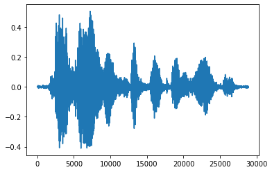
It is more convinient to convert tensor into float numbers and show the audio clip in graph:
import matplotlib.pyplot as plt


tensor = tf.cast(audio_tensor, tf.float32) / 32768.0

plt.figure()
plt.plot(tensor.numpy())
[<matplotlib.lines.Line2D at 0x7fbdd3eb72d0>]
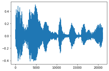
Trim the noise
Sometimes it makes sense to trim the noise from the audio, which could be done through API tfio.audio.trim. Returned from the API is a pair of [start, stop] position of the segement:
position = tfio.audio.trim(tensor, axis=0, epsilon=0.1)
print(position)

start = position[0]
stop = position[1]
print(start, stop)

processed = tensor[start:stop]

plt.figure()
plt.plot(processed.numpy())
tf.Tensor([ 2398 23546], shape=(2,), dtype=int64)
tf.Tensor(2398, shape=(), dtype=int64) tf.Tensor(23546, shape=(), dtype=int64)
[<matplotlib.lines.Line2D at 0x7fbdd3dce9d0>]
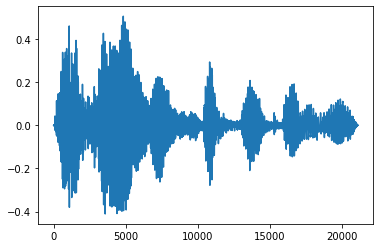
Fade In and Fade Out
One useful audio engineering technique is fade, which gradually increases or decreases audio signals. This can be done through tfio.audio.fade. tfio.audio.fade supports different shapes of fades such as linear, logarithmic, or exponential:
fade = tfio.audio.fade(
    processed, fade_in=1000, fade_out=2000, mode="logarithmic")

plt.figure()
plt.plot(fade.numpy())
[<matplotlib.lines.Line2D at 0x7fbdd00d9b10>]
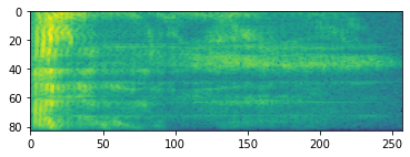
Spectrogram
Advanced audio processing often works on frequency changes over time. In tensorflow-io a waveform can be converted to spectrogram through tfio.audio.spectrogram:
# Convert to spectrogram
spectrogram = tfio.audio.spectrogram(
    fade, nfft=512, window=512, stride=256)

plt.figure()
plt.imshow(tf.math.log(spectrogram).numpy())
<matplotlib.image.AxesImage at 0x7fbdd005add0>
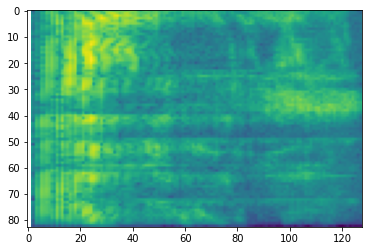
Additional transformation to different scales are also possible:
# Convert to mel-spectrogram
mel_spectrogram = tfio.audio.melscale(
spectrogram, rate=16000, mels=128, fmin=0, fmax=8000)
plt.figure()
plt.imshow(tf.math.log(mel_spectrogram).numpy())
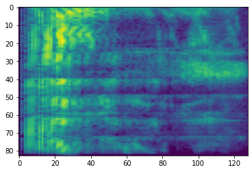
# Convert to db scale mel-spectrogram
dbscale_mel_spectrogram = tfio.audio.dbscale(
mel_spectrogram, top_db=80)
plt.figure()
plt.imshow(dbscale_mel_spectrogram.numpy())
<matplotlib.image.AxesImage at 0x7fbcfb20bd10>
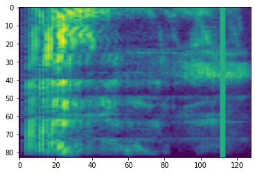
SpecAugment
In addition to the above mentioned data preparation and augmentation APIs, tensorflow-io package also provides advanced spectrogram augmentations, most notably Frequency and Time Masking discussed in SpecAugment: A Simple Data Augmentation Method for Automatic Speech Recognition (Park et al., 2019).
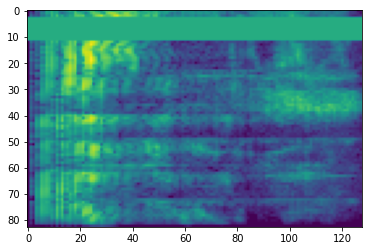
Frequency Masking
In frequency masking, frequency channels [f0, f0 + f) are masked where f is chosen from a uniform distribution from 0 to the frequency mask parameter F, and f0 is chosen from (0, ν − f) where ν is the number of frequency channels.
# Freq masking
freq_mask = tfio.audio.freq_mask(dbscale_mel_spectrogram, param=10)

plt.figure()
plt.imshow(freq_mask.numpy())
<matplotlib.image.AxesImage at 0x7fbcfb155cd0>
Time Masking
In time masking, t consecutive time steps [t0, t0 + t) are masked where t is chosen from a uniform distribution from 0 to the time mask parameter T, and t0 is chosen from [0, τ − t) where τ is the time steps.
# Time masking
time_mask = tfio.audio.time_mask(dbscale_mel_spectrogram, param=10)

plt.figure()
plt.imshow(time_mask.numpy())
<matplotlib.image.AxesImage at 0x7fbcfb0d9bd0>