
| |  GitHubでソースを表示 GitHubでソースを表示 | |
変分推論(VI)は、近似ベイズ推定を最適化問題としてキャストし、真の事後確率とのKL発散を最小化する「代理」事後分布を求めます。勾配ベースのVIは、MCMC法よりも高速であることが多く、モデルパラメータの最適化で自然に構成され、モデル比較、収束診断、および構成可能な推論に直接使用できるモデル証拠の下限を提供します。
TensorFlow Probabilityは、TFPスタックに自然に適合する、高速で柔軟かつスケーラブルなVI用のツールを提供します。これらのツールを使用すると、線形変換またはフローの正規化によって誘導される共分散構造を持つ代理事後確率を構築できます。
VIは、ベイズ推定するために使用することができる信頼性の間隔を関心の結果に様々な処置または観測された機能の効果を推定する回帰モデルのパラメータについて。信頼区間は、観測されたデータを条件とし、パラメーターの事前分布に関する仮定を与えられたパラメーターの事後分布に従って、一定の確率で観測されていないパラメーターの値を制限しました。
(使用して、このコラボでは、我々は、家庭で測定されたラドン濃度の回帰モデル線形ベイズのパラメータのための信頼できる間隔を取得するためにVIを使用する方法を示します。の(2007)ラドンデータセットゲルマンらを参照;同様の例をスタンに)。私たちは、TFP方法を示しJointDistribution sがと組み合わせるbijectors構築し、表情豊かな代理の事後の2種類をフィット:
- ブロック行列によって変換された標準正規分布。行列は、後部のいくつかのコンポーネント間の独立性と他のコンポーネント間の依存性を反映している可能性があり、平均場または完全共分散後部の仮定を緩和します。
- より複雑な、大容量の自己回帰の流れの逆。
サロゲート事後確率はトレーニングされ、平均場サロゲート事後ベースラインからの結果、およびハミルトニアンモンテカルロからのグラウンドトゥルースサンプルと比較されます。
ベイズ変分推論の概要
我々は、以下の生成的プロセスがあると \(\theta\) ランダムパラメータを表し、 \(\omega\) 決定論的パラメータを表し、 \(x_i\) 特徴としている \(y_i\) ための目標値である \(i=1,\ldots,n\) データポイントを観察します:\ begin {ALIGN }&\ theta \ sim r(\ Theta)&& \ text {(Prior)} \&\ text {for} i = 1 \ ldots n:\ nonumber \&\ quad y_i \ sim p(Y_i | x_i、\ theta 、\オメガ)&& \テキスト{(尤度)} \端{ALIGN}
次に、VIは次のように特徴付けられます。$ \ newcommand {\ E} {\ operatorname {\ mathbb {E}}} \ newcommand {\ K} {\ operatorname {\ mathbb {K}}} \ newcommand {\ defeq} {\ overset {\ tiny \ text {def}} {=}} \ DeclareMathOperator * {\ argmin} {arg \、min} $
\ログP({Y_I} _i ^ N | {X_I} _i ^ N、\オメガ) - \ {ALIGN}始める&\ defeq - \ \ INT \ textrm {D} \シータ\、R(\シータ)ログを\ prod_i ^ np(y_i | x_i、\ theta、\ omega)&& \ text {(本当にハードインテグラル)} \&=-\ log \ int \ textrm {d} \ theta \、q(\ theta)\ frac {1 } {q(\ theta)} r(\ theta)\ prod_i ^ np(y_i | x_i、\ theta、\ omega)&& \ text {(1で乗算)} \&\ le- \ int \ textrm {d} \シータ\、Q(\シータ)\ログ\ FRAC {R(\シータ)\ prod_i ^ NP(Y_I | x iは、\シータ、\オメガ)} {Q(\シータ)} && \テキスト{(ジェンセンの不等式)} \&\ defeq \ E {Q(\シータ)} - \ログP(Y_I | X_I、\シータ、\オメガ)] + \ K [Q(\シータ)、R(\シータ)] \& \ defeq \text{expected negative log likelihood"} + \テキスト{KL正則"} \端{ALIGN}
(技術的に我々は想定してい \(q\) ある絶対連続に関して \(r\)。も参照してください、 Jensenの不等式。)
境界はすべてのqに当てはまるため、次の場合は明らかに最も厳しくなります。
\[q^*,w^* = \argmin_{q \in \mathcal{Q},\omega\in\mathbb{R}^d} \left\{ \sum_i^n\E_{q(\Theta)}\left[ -\log p(y_i|x_i,\Theta, \omega) \right] + \K[q(\Theta), r(\Theta)] \right\}\]
用語に関しては、
- \(q^*\) "代理事後"と、
- \(\mathcal{Q}\) "代理家族。"
\(\omega^*\) VI損失に決定論的パラメータの最大尤度値を表します。参照してください。今回の調査変分推論の詳細については、を。
例:ラドン測定でのベイズ階層線形回帰
ラドンは、地面との接点から家に入る放射性ガスです。非喫煙者の肺がんの主な原因は発がん性物質です。ラドンレベルは家庭ごとに大きく異なります。
EPAは、80,000戸の家屋のラドンレベルの調査を行いました。 2つの重要な予測因子は次のとおりです。
- 測定が行われたフロア(地下室のラドンが高い)
- 郡のウランレベル(ラドンレベルとの正の相関)
郡でグループ化された家でラドン濃度を予測することにより導入されたベイズ階層モデルでは古典的な問題であり、ゲルマンとヒル(2006) 。住宅のラドン測定値を予測するための階層線形モデルを構築します。階層は、郡ごとの住宅のグループ化です。ミネソタ州の住宅のラドンレベルに対する場所(郡)の影響の信頼区間に関心があります。この影響を分離するために、床とウランレベルの影響もモデルに含まれています。さらに、測定が行われたフロアの郡ごとに変動がある場合、これは郡の効果に起因しないように、測定が行われた平均フロアに対応するコンテキスト効果を郡ごとに組み込みます。
pip3 install -q tf-nightly tfp-nightly
import matplotlib.pyplot as plt
import numpy as np
import seaborn as sns
import tensorflow as tf
import tensorflow_datasets as tfds
import tensorflow_probability as tfp
import warnings

tfd = tfp.distributions
tfb = tfp.bijectors

plt.rcParams['figure.facecolor'] = '1.'
# Load the Radon dataset from `tensorflow_datasets` and filter to data from
# Minnesota.
dataset = tfds.as_numpy(
    tfds.load('radon', split='train').filter(
        lambda x: x['features']['state'] == 'MN').batch(10**9))

# Dependent variable: Radon measurements by house.
dataset = next(iter(dataset))
radon_measurement = dataset['activity'].astype(np.float32)
radon_measurement[radon_measurement <= 0.] = 0.1
log_radon = np.log(radon_measurement)

# Measured uranium concentrations in surrounding soil.
uranium_measurement = dataset['features']['Uppm'].astype(np.float32)
log_uranium = np.log(uranium_measurement)

# County indicator.
county_strings = dataset['features']['county'].astype('U13')
unique_counties, county = np.unique(county_strings, return_inverse=True)
county = county.astype(np.int32)
num_counties = unique_counties.size

# Floor on which the measurement was taken.
floor_of_house = dataset['features']['floor'].astype(np.int32)

# Average floor by county (contextual effect).
county_mean_floor = []
for i in range(num_counties):
  county_mean_floor.append(floor_of_house[county == i].mean())
county_mean_floor = np.array(county_mean_floor, dtype=log_radon.dtype)
floor_by_county = county_mean_floor[county]
回帰モデルは次のように指定されます。
\(\newcommand{\Normal}{\operatorname{\sf Normal} }\)\開始{ALIGN}&\テキスト{uranium_weight} \ SIM \ノーマル(0、1)\&\テキスト{county_floor_weight} \ SIM \ノーマル(0、1)\&\ J = 1 {用}テキスト\ ldots \ text {num_counties}:\&\ quad \ text {county_effect} _j \ sim \ Normal(0、\ sigma_c)\&\ text {for} i = 1 \ ldots n:\&\ quad \ mu_i =(\ &\カッド\カッド\テキスト{バイアス} \&\カッド\クワッド+ \テキスト{郡の効果} {\テキスト{郡} _i} \&\カッド\クワッド+ \テキスト{log_uranium} _i \回\テキスト{uranium_weight } \&\カッド\クワッド+ \テキスト{floor_of_house} _i \回\テキスト{floor_weight} \&\カッド\クワッド+ \テキスト{floor_by郡} {\テキスト{郡} _i} \回\テキスト{county_floor_weight}) \&\クワッド\テキスト{log_radon} _i(\ sigma_y \ mu_i)\端{ALIGN}た通常\ SIM \ \(i\) インデックス観察と \(\text{county}_i\) 郡である \(i\)番目の観測でした取られた。
郡レベルのランダム効果を使用して、地理的な変動をキャプチャします。パラメータはuranium_weightとcounty_floor_weight確率的モデル化され、そしてfloor_weightと一定のbias決定論的です。これらのモデリングの選択は主に任意であり、合理的な複雑さの確率モデルでVIを示すことを目的としています。 TFPで固定とランダム効果を持つマルチレベルモデリングのより完全な議論については、ラドンデータセットを使用して、参照のマルチレベルのモデリング入門と変分推論を用いてフィッティング一般化線形混合効果モデルを。
# Create variables for fixed effects.
floor_weight = tf.Variable(0.)
bias = tf.Variable(0.)

# Variables for scale parameters.
log_radon_scale = tfp.util.TransformedVariable(1., tfb.Exp())
county_effect_scale = tfp.util.TransformedVariable(1., tfb.Exp())

# Define the probabilistic graphical model as a JointDistribution.
@tfd.JointDistributionCoroutineAutoBatched
def model():
  uranium_weight = yield tfd.Normal(0., scale=1., name='uranium_weight')
  county_floor_weight = yield tfd.Normal(
      0., scale=1., name='county_floor_weight')
  county_effect = yield tfd.Sample(
      tfd.Normal(0., scale=county_effect_scale),
      sample_shape=[num_counties], name='county_effect')
  yield tfd.Normal(
      loc=(log_uranium * uranium_weight + floor_of_house* floor_weight
           + floor_by_county * county_floor_weight
           + tf.gather(county_effect, county, axis=-1)
           + bias),
      scale=log_radon_scale[..., tf.newaxis],
      name='log_radon')

# Pin the observed `log_radon` values to model the un-normalized posterior.
target_model = model.experimental_pin(log_radon=log_radon)
表現力豊かな代理事後確率
次に、2つの異なるタイプの代理事後確率でVIを使用して、ランダム効果の事後分布を推定します。
- ブロック単位の行列変換によって誘導された共分散構造を持つ、制約付きの多変量正規分布。
- 形質転換多変量標準正規分布の逆自己回帰フロー次いで分割および後方の支持と一致するように再構成され、。
多変量正規代理後部
この代理後部を構築するために、訓練可能な線形演算子を使用して、後部のコンポーネント間の相関を誘導します。
# Determine the `event_shape` of the posterior, and calculate the size of each
# `event_shape` component. These determine the sizes of the components of the
# underlying standard Normal distribution, and the dimensions of the blocks in
# the blockwise matrix transformation.
event_shape = target_model.event_shape_tensor()
flat_event_shape = tf.nest.flatten(event_shape)
flat_event_size = tf.nest.map_structure(tf.reduce_prod, flat_event_shape)

# The `event_space_bijector` maps unconstrained values (in R^n) to the support
# of the prior -- we'll need this at the end to constrain Multivariate Normal
# samples to the prior's support.
event_space_bijector = target_model.experimental_default_event_space_bijector()
構築JointDistribution対応する事前構成要素によって決定サイズのベクトル値の標準正規成分とを、。線形演算子で変換できるように、コンポーネントはベクトル値である必要があります。
base_standard_dist = tfd.JointDistributionSequential(
      [tfd.Sample(tfd.Normal(0., 1.), s) for s in flat_event_size])
トレーニング可能なブロックワイズ下三角線形演算子を作成します。これを標準正規分布に適用して、(トレーニング可能な)ブロック単位の行列変換を実装し、後部の相関構造を誘導します。
オペレータ線形ブロック単位内で、訓練可能なフルマトリクスブロックは、ゼロ(またはブロックしながら、後部の2つの構成要素間の完全な共分散を表すNone )を発現する独立。対角上のブロックは下三角行列または対角行列のいずれかであるため、ブロック構造全体が下三角行列を表します。
このバイジェクターを基本分布に適用すると、平均が0で、(コレスキー分解された)共分散が下三角ブロック行列に等しい多変量正規分布になります。
operators = (
    (tf.linalg.LinearOperatorDiag,),  # Variance of uranium weight (scalar).
    (tf.linalg.LinearOperatorFullMatrix,  # Covariance between uranium and floor-by-county weights.
     tf.linalg.LinearOperatorDiag),  # Variance of floor-by-county weight (scalar).
    (None,  # Independence between uranium weight and county effects.
     None,  #  Independence between floor-by-county and county effects.
     tf.linalg.LinearOperatorDiag)  # Independence among the 85 county effects.
    )

block_tril_linop = (
    tfp.experimental.vi.util.build_trainable_linear_operator_block(
        operators, flat_event_size))
scale_bijector = tfb.ScaleMatvecLinearOperatorBlock(block_tril_linop)
標準正規分布に線形演算子を適用した後、マルチパート適用Shift平均はゼロ以外の値を取ることができるようにbijectorを。
loc_bijector = tfb.JointMap(
    tf.nest.map_structure(
        lambda s: tfb.Shift(
            tf.Variable(tf.random.uniform(
                (s,), minval=-2., maxval=2., dtype=tf.float32))),
        flat_event_size))
スケールと位置のバイジェクターを使用して標準正規分布を変換することによって得られる、結果の多変量正規分布は、事前分布に一致するように再形成および再構築し、最終的に事前分布のサポートに制約する必要があります。
# Reshape each component to match the prior, using a nested structure of
# `Reshape` bijectors wrapped in `JointMap` to form a multipart bijector.
reshape_bijector = tfb.JointMap(
    tf.nest.map_structure(tfb.Reshape, flat_event_shape))

# Restructure the flat list of components to match the prior's structure
unflatten_bijector = tfb.Restructure(
        tf.nest.pack_sequence_as(
            event_shape, range(len(flat_event_shape))))
ここで、すべてをまとめます。トレーニング可能なバイジェクターをチェーンし、それらを基本標準正規分布に適用して、代理後部を構築します。
surrogate_posterior = tfd.TransformedDistribution(
    base_standard_dist,
    bijector = tfb.Chain(  # Note that the chained bijectors are applied in reverse order
        [
         event_space_bijector,  # constrain the surrogate to the support of the prior
         unflatten_bijector,  # pack the reshaped components into the `event_shape` structure of the posterior
         reshape_bijector,  # reshape the vector-valued components to match the shapes of the posterior components
         loc_bijector,  # allow for nonzero mean
         scale_bijector  # apply the block matrix transformation to the standard Normal distribution
         ]))
多変量正規代理後部をトレーニングします。
optimizer = tf.optimizers.Adam(learning_rate=1e-2)
mvn_loss = tfp.vi.fit_surrogate_posterior(
target_model.unnormalized_log_prob,
surrogate_posterior,
optimizer=optimizer,
num_steps=10**4,
sample_size=16,
jit_compile=True)
mvn_samples = surrogate_posterior.sample(1000)
mvn_final_elbo = tf.reduce_mean(
target_model.unnormalized_log_prob(*mvn_samples)
- surrogate_posterior.log_prob(mvn_samples))
print('Multivariate Normal surrogate posterior ELBO: {}'.format(mvn_final_elbo))
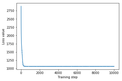
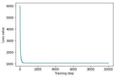
plt.plot(mvn_loss)
plt.xlabel('Training step')
_ = plt.ylabel('Loss value')
Multivariate Normal surrogate posterior ELBO: -1065.705322265625
トレーニングされた代理事後確率はTFP分布であるため、そこからサンプルを取得して処理し、パラメーターの事後信頼区間を生成できます。
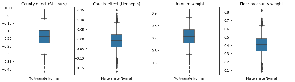
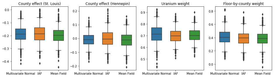
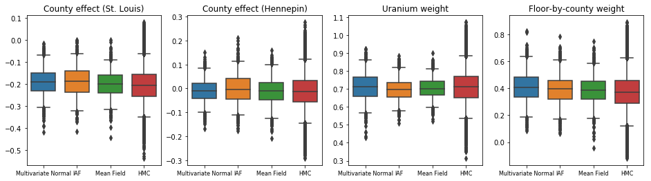
ショー50%および95%の下のボックスアンドウィスカープロット信頼区間土壌ウランの測定及び郡による平均フロア上の2つの最大の郡と回帰重みの郡効果について。郡の影響に関する後の信頼区間は、セントルイス郡の場所が他の変数を考慮した後、より低いラドンレベルに関連付けられていること、およびヘネピン郡の場所の影響がほぼ中立であることを示しています。
回帰重みの事後信頼区間は、土壌ウランのレベルが高いほどラドンレベルが高くなることを示しており、高層階で測定が行われた郡(家に地下室がなかったためと思われる)ではラドンレベルが高くなる傾向があります。これは、土壌の特性と、建設された構造物のタイプに対するそれらの影響に関連している可能性があります。
床の(決定論的)係数は負であり、予想どおり、床が低いほどラドンレベルが高いことを示しています。
st_louis_co = 69  # Index of St. Louis, the county with the most observations.
hennepin_co = 25  # Index of Hennepin, with the second-most observations.

def pack_samples(samples):
  return {'County effect (St. Louis)': samples.county_effect[..., st_louis_co],
          'County effect (Hennepin)': samples.county_effect[..., hennepin_co],
          'Uranium weight': samples.uranium_weight,
          'Floor-by-county weight': samples.county_floor_weight}

def plot_boxplot(posterior_samples):
  fig, axes = plt.subplots(1, 4, figsize=(16, 4))

  # Invert the results dict for easier plotting.
  k = list(posterior_samples.values())[0].keys()
  plot_results = {
      v: {p: posterior_samples[p][v] for p in posterior_samples} for v in k}
  for i, (var, var_results) in enumerate(plot_results.items()):
    sns.boxplot(data=list(var_results.values()), ax=axes[i],
                width=0.18*len(var_results), whis=(2.5, 97.5))
    # axes[i].boxplot(list(var_results.values()), whis=(2.5, 97.5))
    axes[i].title.set_text(var)
    fs = 10 if len(var_results) < 4 else 8
    axes[i].set_xticklabels(list(var_results.keys()), fontsize=fs)

results = {'Multivariate Normal': pack_samples(mvn_samples)}

print('Bias is: {:.2f}'.format(bias.numpy()))
print('Floor fixed effect is: {:.2f}'.format(floor_weight.numpy()))
plot_boxplot(results)
Bias is: 1.40
Floor fixed effect is: -0.72
逆自己回帰フローサロゲート後方
逆自己回帰フロー(IAF)は、ニューラルネットワークを使用して分布のコンポーネント間の複雑な非線形依存関係をキャプチャする正規化フローです。次に、IAFサロゲートを後方に構築して、この大容量で柔軟性の高いモデルが制約付き多変量正規分布よりも優れているかどうかを確認します。
# Build a standard Normal with a vector `event_shape`, with length equal to the
# total number of degrees of freedom in the posterior.
base_distribution = tfd.Sample(
    tfd.Normal(0., 1.), sample_shape=[tf.reduce_sum(flat_event_size)])

# Apply an IAF to the base distribution.
num_iafs = 2
iaf_bijectors = [
    tfb.Invert(tfb.MaskedAutoregressiveFlow(
        shift_and_log_scale_fn=tfb.AutoregressiveNetwork(
            params=2, hidden_units=[256, 256], activation='relu')))
    for _ in range(num_iafs)
]

# Split the base distribution's `event_shape` into components that are equal
# in size to the prior's components.
split = tfb.Split(flat_event_size)

# Chain these bijectors and apply them to the standard Normal base distribution
# to build the surrogate posterior. `event_space_bijector`,
# `unflatten_bijector`, and `reshape_bijector` are the same as in the
# multivariate Normal surrogate posterior.
iaf_surrogate_posterior = tfd.TransformedDistribution(
    base_distribution,
    bijector=tfb.Chain([
         event_space_bijector,  # constrain the surrogate to the support of the prior
         unflatten_bijector,  # pack the reshaped components into the `event_shape` structure of the prior
         reshape_bijector,  # reshape the vector-valued components to match the shapes of the prior components
         split] +  # Split the samples into components of the same size as the prior components
         iaf_bijectors  # Apply a flow model to the Tensor-valued standard Normal distribution
         ))
IAF代理を後方に訓練します。
optimizer=tf.optimizers.Adam(learning_rate=1e-2)
iaf_loss = tfp.vi.fit_surrogate_posterior(
target_model.unnormalized_log_prob,
iaf_surrogate_posterior,
optimizer=optimizer,
num_steps=10**4,
sample_size=4,
jit_compile=True)
iaf_samples = iaf_surrogate_posterior.sample(1000)
iaf_final_elbo = tf.reduce_mean(
target_model.unnormalized_log_prob(*iaf_samples)
- iaf_surrogate_posterior.log_prob(iaf_samples))
print('IAF surrogate posterior ELBO: {}'.format(iaf_final_elbo))
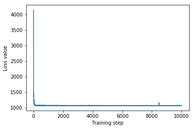
plt.plot(iaf_loss)
plt.xlabel('Training step')
_ = plt.ylabel('Loss value')
IAF surrogate posterior ELBO: -1065.3663330078125
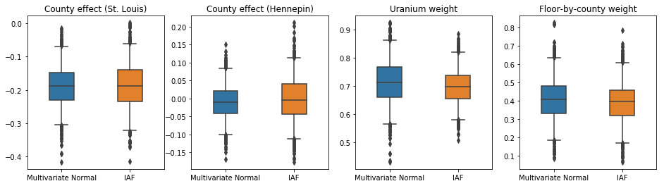
IAF代理事後確率の信頼区間は、制約付き多変量正規分布の区間と同様に見えます。
results['IAF'] = pack_samples(iaf_samples)
plot_boxplot(results)
ベースライン:平均場代理後部
VIの代理事後確率は、訓練可能な平均と分散を備えた平均場(独立)正規分布であると見なされることが多く、全単射変換による事前分布のサポートに制約されます。多変量正規代理事後確率と同じ一般式を使用して、2つのより表現力豊かな代理出産事後確率に加えて、平均場代理出産事後確率を定義します。
# A block-diagonal linear operator, in which each block is a diagonal operator,
# transforms the standard Normal base distribution to produce a mean-field
# surrogate posterior.
operators = (tf.linalg.LinearOperatorDiag,
             tf.linalg.LinearOperatorDiag,
             tf.linalg.LinearOperatorDiag)
block_diag_linop = (
    tfp.experimental.vi.util.build_trainable_linear_operator_block(
        operators, flat_event_size))
mean_field_scale = tfb.ScaleMatvecLinearOperatorBlock(block_diag_linop)

mean_field_loc = tfb.JointMap(
    tf.nest.map_structure(
        lambda s: tfb.Shift(
            tf.Variable(tf.random.uniform(
                (s,), minval=-2., maxval=2., dtype=tf.float32))),
        flat_event_size))

mean_field_surrogate_posterior = tfd.TransformedDistribution(
    base_standard_dist,
    bijector = tfb.Chain(  # Note that the chained bijectors are applied in reverse order
        [
         event_space_bijector,  # constrain the surrogate to the support of the prior
         unflatten_bijector,  # pack the reshaped components into the `event_shape` structure of the posterior
         reshape_bijector, # reshape the vector-valued components to match the shapes of the posterior components
         mean_field_loc,   # allow for nonzero mean
         mean_field_scale  # apply the block matrix transformation to the standard Normal distribution
         ]))

optimizer=tf.optimizers.Adam(learning_rate=1e-2)
mean_field_loss = tfp.vi.fit_surrogate_posterior(
    target_model.unnormalized_log_prob,
    mean_field_surrogate_posterior,
    optimizer=optimizer,
    num_steps=10**4,
    sample_size=16,
    jit_compile=True)

mean_field_samples = mean_field_surrogate_posterior.sample(1000)
mean_field_final_elbo = tf.reduce_mean(
    target_model.unnormalized_log_prob(*mean_field_samples)
    - mean_field_surrogate_posterior.log_prob(mean_field_samples))
print('Mean-field surrogate posterior ELBO: {}'.format(mean_field_final_elbo))

plt.plot(mean_field_loss)
plt.xlabel('Training step')
_ = plt.ylabel('Loss value')
Mean-field surrogate posterior ELBO: -1065.7652587890625
この場合、平均場代理事後確率は、より表現力のある代理出産事後確率と同様の結果をもたらし、この単純なモデルが推論タスクに適している可能性があることを示しています。
results['Mean Field'] = pack_samples(mean_field_samples)
plot_boxplot(results)
グラウンドトゥルース:ハミルトニアンモンテカルロ(HMC)
HMCを使用して、代理事後確率の結果と比較するために、真の事後確率から「グラウンドトゥルース」サンプルを生成します。
num_chains = 8
num_leapfrog_steps = 3
step_size = 0.4
num_steps=20000

flat_event_shape = tf.nest.flatten(target_model.event_shape)
enum_components = list(range(len(flat_event_shape)))
bijector = tfb.Restructure(
    enum_components,
    tf.nest.pack_sequence_as(target_model.event_shape, enum_components))(
        target_model.experimental_default_event_space_bijector())

current_state = bijector(
    tf.nest.map_structure(
        lambda e: tf.zeros([num_chains] + list(e), dtype=tf.float32),
    target_model.event_shape))

hmc = tfp.mcmc.HamiltonianMonteCarlo(
    target_log_prob_fn=target_model.unnormalized_log_prob,
    num_leapfrog_steps=num_leapfrog_steps,
    step_size=[tf.fill(s.shape, step_size) for s in current_state])

hmc = tfp.mcmc.TransformedTransitionKernel(
    hmc, bijector)
hmc = tfp.mcmc.DualAveragingStepSizeAdaptation(
    hmc,
    num_adaptation_steps=int(num_steps // 2 * 0.8),
    target_accept_prob=0.9)

chain, is_accepted = tf.function(
    lambda current_state: tfp.mcmc.sample_chain(
        current_state=current_state,
        kernel=hmc,
        num_results=num_steps // 2,
        num_burnin_steps=num_steps // 2,
        trace_fn=lambda _, pkr:
        (pkr.inner_results.inner_results.is_accepted),
        ),
    autograph=False,
    jit_compile=True)(current_state)

accept_rate = tf.reduce_mean(tf.cast(is_accepted, tf.float32))
ess = tf.nest.map_structure(
    lambda c: tfp.mcmc.effective_sample_size(
        c,
        cross_chain_dims=1,
        filter_beyond_positive_pairs=True),
    chain)

r_hat = tf.nest.map_structure(tfp.mcmc.potential_scale_reduction, chain)
hmc_samples = pack_samples(
    tf.nest.pack_sequence_as(target_model.event_shape, chain))
print('Acceptance rate is {}'.format(accept_rate))
Acceptance rate is 0.9008625149726868
サンプルトレースを健全性チェックにプロットします。HMCの結果を確認します。
def plot_traces(var_name, samples):
  fig, axes = plt.subplots(1, 2, figsize=(14, 1.5), sharex='col', sharey='col')
  for chain in range(num_chains):
    s = samples.numpy()[:, chain]
    axes[0].plot(s, alpha=0.7)
    sns.kdeplot(s, ax=axes[1], shade=False)
    axes[0].title.set_text("'{}' trace".format(var_name))
    axes[1].title.set_text("'{}' distribution".format(var_name))
    axes[0].set_xlabel('Iteration')

warnings.filterwarnings('ignore')
for var, var_samples in hmc_samples.items():
  plot_traces(var, var_samples)
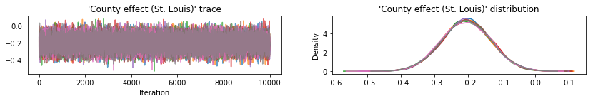
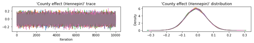
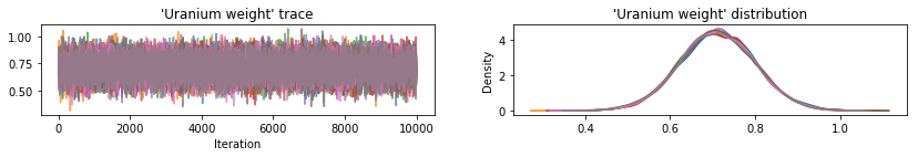
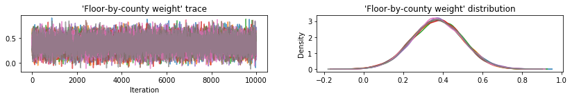
3つの代理事後確率はすべて、HMCサンプルと視覚的に類似した信頼区間を生成しましたが、VIで一般的であるように、ELBO損失の影響により分散が不十分な場合があります。
results['HMC'] = hmc_samples
plot_boxplot(results)
追加の結果
プロット関数
plt.rcParams.update({'axes.titlesize': 'medium', 'xtick.labelsize': 'medium'})
def plot_loss_and_elbo():
  fig, axes = plt.subplots(1, 2, figsize=(12, 4))

  axes[0].scatter([0, 1, 2],
                  [mvn_final_elbo.numpy(),
                  iaf_final_elbo.numpy(),
                  mean_field_final_elbo.numpy()])
  axes[0].set_xticks(ticks=[0, 1, 2])
  axes[0].set_xticklabels(labels=[
    'Multivariate Normal', 'IAF', 'Mean Field'])
  axes[0].title.set_text('Evidence Lower Bound (ELBO)')

  axes[1].plot(mvn_loss, label='Multivariate Normal')
  axes[1].plot(iaf_loss, label='IAF')
  axes[1].plot(mean_field_loss, label='Mean Field')
  axes[1].set_ylim([1000, 4000])
  axes[1].set_xlabel('Training step')
  axes[1].set_ylabel('Loss (negative ELBO)')
  axes[1].title.set_text('Loss')
  plt.legend()
  plt.show()

plt.rcParams.update({'axes.titlesize': 'medium', 'xtick.labelsize': 'small'})
def plot_kdes(num_chains=8):
  fig, axes = plt.subplots(2, 2, figsize=(12, 8))
  k = list(results.values())[0].keys()
  plot_results = {
      v: {p: results[p][v] for p in results} for v in k}
  for i, (var, var_results) in enumerate(plot_results.items()):
    ax = axes[i % 2, i // 2]
    for posterior, posterior_results in var_results.items():
      if posterior == 'HMC':
        label = posterior
        for chain in range(num_chains):
          sns.kdeplot(
              posterior_results[:, chain],
              ax=ax, shade=False, color='k', linestyle=':', label=label)
          label=None
      else:
        sns.kdeplot(
            posterior_results, ax=ax, shade=False, label=posterior)
        ax.title.set_text('{}'.format(var))
    ax.legend()
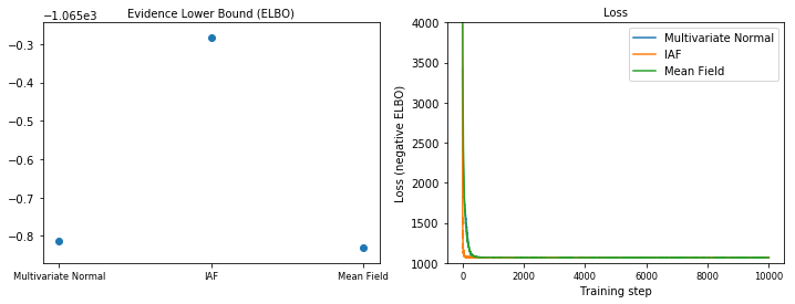
証拠下限(ELBO)
IAFは、はるかに大きく、最も柔軟なサロゲート事後確率であり、最も高いエビデンス下限(ELBO)に収束します。
plot_loss_and_elbo()
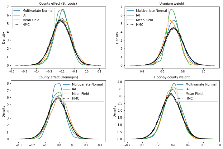
後方サンプル
HMCグラウンドトゥルースサンプルと比較した、各サロゲート後方からのサンプル(箱ひげ図に示されているサンプルの異なる視覚化)。
plot_kdes()
結論
このコラボでは、同時分布とマルチパートバイジェクターを使用してVI代理事後確率を作成し、それらを適合させて、ラドンデータセットの回帰モデルの重みの信頼区間を推定しました。この単純なモデルの場合、より表現力のある代理事後確率は、平均場代理出産事後確率と同様に実行されます。ただし、ここで示したツールを使用して、より複雑なモデルに適したさまざまな柔軟な代理事後確率を構築できます。