GitHub でソースを表示{ GitHub でソースを表示{ |
このチュートリアルでは、簡略化された MNIST バージョンを分類する、Farhi et al で使用されたアプローチに似た量子ニューラルネットワーク(QNN)を構築し、古典的なデータ問題における量子ニューラルネットワークのパフォーマンスを従来のニューラルネットワークと比較します。
セットアップ
pip install -q tensorflow==2.3.1TensorFlow Quantum をインストールします。
pip install -q tensorflow-quantum次に、TensorFlow とモジュールの依存関係をインポートします。
import tensorflow as tf
import tensorflow_quantum as tfq

import cirq
import sympy
import numpy as np
import seaborn as sns
import collections

# visualization tools
%matplotlib inline
import matplotlib.pyplot as plt
from cirq.contrib.svg import SVGCircuit
1. データを読み込む
このチュートリアルでは、Farhi et al. に従って、数字の 3 と 6 を区別する二項分類器を構築します。このセクションでは、次を行うデータ処理を説明します。
- Keras から生データを読み込みます。
- データセットを 3 と 6 に絞り込みます。
- 画像が量子コンピュータに適合するように、画像を縮小します。
- 矛盾するサンプルを取り除きます。
- バイナリ画像を Cirq 回路に変換します。
- Cirq 回路を TensorFlow Quantum 回路に変換します。
1.1 生データを読み込む
Keras で配布された MNIST データセットを読み込みます。
(x_train, y_train), (x_test, y_test) = tf.keras.datasets.mnist.load_data()

# Rescale the images from [0,255] to the [0.0,1.0] range.
x_train, x_test = x_train[..., np.newaxis]/255.0, x_test[..., np.newaxis]/255.0

print("Number of original training examples:", len(x_train))
print("Number of original test examples:", len(x_test))
Number of original training examples: 60000
Number of original test examples: 10000
3 と 6 の数字のみを保持してほかのクラスを取り除くように、データセットを絞り込みます。同時に、3 を True、6 を False というように、ラベル y をブール型に変換します。
def filter_36(x, y):
    keep = (y == 3) | (y == 6)
    x, y = x[keep], y[keep]
    y = y == 3
    return x,y
x_train, y_train = filter_36(x_train, y_train)
x_test, y_test = filter_36(x_test, y_test)

print("Number of filtered training examples:", len(x_train))
print("Number of filtered test examples:", len(x_test))
Number of filtered training examples: 12049
Number of filtered test examples: 1968
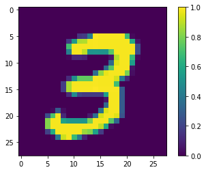
最初のサンプルを表示します。
print(y_train[0])

plt.imshow(x_train[0, :, :, 0])
plt.colorbar()
True
<matplotlib.colorbar.Colorbar at 0x7fd20ebb9978>
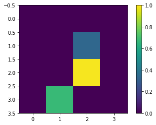
1.2 画像を縮小する
現在の量子コンピュータでは、画像サイズ 28x28 は大きすぎるため、4x4 に縮小します。
x_train_small = tf.image.resize(x_train, (4,4)).numpy()
x_test_small = tf.image.resize(x_test, (4,4)).numpy()
サイズ変更を行ったら、もう一度最初のサンプルを表示します。
print(y_train[0])

plt.imshow(x_train_small[0,:,:,0], vmin=0, vmax=1)
plt.colorbar()
True
<matplotlib.colorbar.Colorbar at 0x7fd18c24c780>
1.3 矛盾するサンプルを取り除く
Farhi et al. の 3.3 Learning to Distinguish Digits セクションに説明されているように、データセットから両方のクラスに属するラベルが付けられた画像を取り除きます。
これは標準的な機械学習の手順ではありませんが、論文の手順に従う目的で追加している手順です。
def remove_contradicting(xs, ys):
    mapping = collections.defaultdict(set)
    # Determine the set of labels for each unique image:
    for x,y in zip(xs,ys):
       mapping[tuple(x.flatten())].add(y)

    new_x = []
    new_y = []
    for x,y in zip(xs, ys):
      labels = mapping[tuple(x.flatten())]
      if len(labels) == 1:
          new_x.append(x)
          new_y.append(list(labels)[0])
      else:
          # Throw out images that match more than one label.
          pass

    num_3 = sum(1 for value in mapping.values() if True in value)
    num_6 = sum(1 for value in mapping.values() if False in value)
    num_both = sum(1 for value in mapping.values() if len(value) == 2)

    print("Number of unique images:", len(mapping.values()))
    print("Number of 3s: ", num_3)
    print("Number of 6s: ", num_6)
    print("Number of contradictory images: ", num_both)
    print()
    print("Initial number of examples: ", len(xs))
    print("Remaining non-contradictory examples: ", len(new_x))

    return np.array(new_x), np.array(new_y)
取り除いた結果の数量は、レポートされている値に密に一致していませんが、これは正確な手順が指定されていないためです。
また、この時点で、矛盾するサンプルをフィルタリングすることで、矛盾するトレーニングサンプルがモデルに絶対に送られないということではありません。次のデータの二項化のステップでは、さらに競合が発生します。
x_train_nocon, y_train_nocon = remove_contradicting(x_train_small, y_train)
Number of unique images: 10387
Number of 3s:  4961
Number of 6s:  5475
Number of contradictory images:  49

Initial number of examples:  12049
Remaining non-contradictory examples:  11520
1.3 データを量子回路としてエンコードする
Farhi et al. は、量子コンピュータを使って画像を処理するには、ピクセルの値に応じた状態で、各ピクセルをキュービットで表現するように提案しています。最初のステップでは、バイナリエンコーディングへの変換を行います。
THRESHOLD = 0.5

x_train_bin = np.array(x_train_nocon > THRESHOLD, dtype=np.float32)
x_test_bin = np.array(x_test_small > THRESHOLD, dtype=np.float32)
この時点で矛盾した画像を取り除く場合、193 個しか画像が残らず、これでは有効なトレーニングを行える数量とは言えません。
_ = remove_contradicting(x_train_bin, y_train_nocon)
Number of unique images: 193
Number of 3s:  124
Number of 6s:  113
Number of contradictory images:  44

Initial number of examples:  11520
Remaining non-contradictory examples:  3731
しきい値を超える値を持つピクセルインデックスのキュービットは、\(X\) ゲートを介して循環します。
def convert_to_circuit(image):
    """Encode truncated classical image into quantum datapoint."""
    values = np.ndarray.flatten(image)
    qubits = cirq.GridQubit.rect(4, 4)
    circuit = cirq.Circuit()
    for i, value in enumerate(values):
        if value:
            circuit.append(cirq.X(qubits[i]))
    return circuit


x_train_circ = [convert_to_circuit(x) for x in x_train_bin]
x_test_circ = [convert_to_circuit(x) for x in x_test_bin]
これは最初のサンプルに作成された回路です(回路図には、ゼロゲートのキュービットは表示されていません)。
SVGCircuit(x_train_circ[0])
findfont: Font family ['Arial'] not found. Falling back to DejaVu Sans.

この回路を、画像の値がしきい値を超えるインデックスを比較します。
bin_img = x_train_bin[0,:,:,0]
indices = np.array(np.where(bin_img)).T
indices
array([[2, 2],
       [3, 1]])
これらの Cirq 回路を tfq のテンソルに変換します。
x_train_tfcirc = tfq.convert_to_tensor(x_train_circ)
x_test_tfcirc = tfq.convert_to_tensor(x_test_circ)
2. 量子ニューラルネットワーク
画像を分類する量子回路構造に関するガイダンスはほとんどありません。分類は読み出されるキュービットの期待に基づいて行われるため、Farhi et al. は、2 つのキュービットゲートを使用して、読み出しキュービットが必ず作用されるようにすることを提案しています。これはある意味、ピクセル全体に小さなユニタリ RNNを実行することに似ています。
2.1 モデル回路を構築する
次の例では、このレイヤー化アプローチを説明しています。各レイヤーは同一ゲートの n 個のインスタンスを使用しており、各データキュービットは読み出しキュービットに影響を与えています。
ゲートのレイヤーを回路に追加する簡単なクラスから始めましょう。
class CircuitLayerBuilder():
    def __init__(self, data_qubits, readout):
        self.data_qubits = data_qubits
        self.readout = readout

    def add_layer(self, circuit, gate, prefix):
        for i, qubit in enumerate(self.data_qubits):
            symbol = sympy.Symbol(prefix + '-' + str(i))
            circuit.append(gate(qubit, self.readout)**symbol)
サンプル回路レイヤーを構築して、どのようになるかを確認します。
demo_builder = CircuitLayerBuilder(data_qubits = cirq.GridQubit.rect(4,1),
                                   readout=cirq.GridQubit(-1,-1))

circuit = cirq.Circuit()
demo_builder.add_layer(circuit, gate = cirq.XX, prefix='xx')
SVGCircuit(circuit)

では、2 レイヤーモデルを構築しましょう。 データ回路サイズに一致するようにし、準備と読み出し演算を含めます。
def create_quantum_model():
    """Create a QNN model circuit and readout operation to go along with it."""
    data_qubits = cirq.GridQubit.rect(4, 4)  # a 4x4 grid.
    readout = cirq.GridQubit(-1, -1)         # a single qubit at [-1,-1]
    circuit = cirq.Circuit()

    # Prepare the readout qubit.
    circuit.append(cirq.X(readout))
    circuit.append(cirq.H(readout))

    builder = CircuitLayerBuilder(
        data_qubits = data_qubits,
        readout=readout)

    # Then add layers (experiment by adding more).
    builder.add_layer(circuit, cirq.XX, "xx1")
    builder.add_layer(circuit, cirq.ZZ, "zz1")

    # Finally, prepare the readout qubit.
    circuit.append(cirq.H(readout))

    return circuit, cirq.Z(readout)
model_circuit, model_readout = create_quantum_model()
2.2 tfq-keras モデルでモデル回路をラップする
量子コンポーネントで Keras モデルを構築します。このモデルには、古典的なデータをエンコードする「量子データ」が x_train_circ からフィードされます。パラメータ化された量子回路レイヤーの tfq.layers.PQC を使用して、量子データでモデル回路をトレーニングするモデルです。
Farhi et al. は、画像を分類するには、パラメータ化された回路で読み出しキュービットの期待値を使用することを提案しています。期待値は、1 から -1 の値です。
# Build the Keras model.
model = tf.keras.Sequential([
    # The input is the data-circuit, encoded as a tf.string
    tf.keras.layers.Input(shape=(), dtype=tf.string),
    # The PQC layer returns the expected value of the readout gate, range [-1,1].
    tfq.layers.PQC(model_circuit, model_readout),
])
次に、compile メソッドを使用して、モデルにトレーニング手順を指定します。
期待される読み出しは [-1,1] の範囲であるため、ヒンジ損失を最適化すると、ある程度自然な適合となります。
注意: もう 1 つの有効なアプローチとして、出力範囲を [0,1] にシフトし、モデルがクラス 3 に割りてる確率として扱う方法があります。これは、標準的なtf.losses.BinaryCrossentropy 損失で使用することができます。
ここでヒンジ損失を使用するには、小さな調整を 2 つ行う必要があります。まず、ラベル y_train_nocon をブール型からヒンジ損失が期待する [-1,1] に変換することです。
y_train_hinge = 2.0*y_train_nocon-1.0
y_test_hinge = 2.0*y_test-1.0
次に、[-1, 1] を y_true ラベル引数として正しく処理するカスタムの hinge_accuracy メトリックを使用します。tf.losses.BinaryAccuracy(threshold=0.0) は y_true がブール型であることを期待するため、ヒンジ損失とは使用できません。
def hinge_accuracy(y_true, y_pred):
    y_true = tf.squeeze(y_true) > 0.0
    y_pred = tf.squeeze(y_pred) > 0.0
    result = tf.cast(y_true == y_pred, tf.float32)

    return tf.reduce_mean(result)
model.compile(
    loss=tf.keras.losses.Hinge(),
    optimizer=tf.keras.optimizers.Adam(),
    metrics=[hinge_accuracy])
print(model.summary())
Model: "sequential"
_________________________________________________________________
Layer (type)                 Output Shape              Param #
=================================================================
pqc (PQC)                    (None, 1)                 32
=================================================================
Total params: 32
Trainable params: 32
Non-trainable params: 0
_________________________________________________________________
None
量子モデルをトレーニングする
では、モデルをトレーニングしましょう。これには約 45 分かかりますが、その時間を待てない方は、小規模なデータのサブセット(以下のNUM_EXAMPLES=500 セット)を使用するとよいでしょう。トレーニング時のモデルの進捗にあまり影響はありません(パラメータは 32 しかなく、これらを制約する上であまりデータは必要ありません)。サンプル数を減らすことでトレーニングを早めに(5 分程度)終わらせることができますが、検証ログに進捗状況を示すには十分な長さです。
EPOCHS = 3
BATCH_SIZE = 32

NUM_EXAMPLES = len(x_train_tfcirc)
x_train_tfcirc_sub = x_train_tfcirc[:NUM_EXAMPLES]
y_train_hinge_sub = y_train_hinge[:NUM_EXAMPLES]
このモデルを収束までトレーニングすると、テストセットにおいて 85% を超える精度が達成されます。
qnn_history = model.fit(
      x_train_tfcirc_sub, y_train_hinge_sub,
      batch_size=32,
      epochs=EPOCHS,
      verbose=1,
      validation_data=(x_test_tfcirc, y_test_hinge))

qnn_results = model.evaluate(x_test_tfcirc, y_test)
Epoch 1/3
360/360 [==============================] - 157s 437ms/step - loss: 0.6086 - hinge_accuracy: 0.8227 - val_loss: 0.3569 - val_hinge_accuracy: 0.8992
Epoch 2/3
360/360 [==============================] - 154s 427ms/step - loss: 0.3384 - hinge_accuracy: 0.8885 - val_loss: 0.3415 - val_hinge_accuracy: 0.8634
Epoch 3/3
360/360 [==============================] - 161s 447ms/step - loss: 0.3349 - hinge_accuracy: 0.8806 - val_loss: 0.3409 - val_hinge_accuracy: 0.8649
62/62 [==============================] - 4s 71ms/step - loss: 0.3409 - hinge_accuracy: 0.8649
注意: トレーニング精度はエポックの平均値を示します。検証精度はエポックの終了ごとに評価されます。
3. 従来のニューラルネットワーク
量子ニューラルネットワークは、この単純化された MNIST 問題で機能するものの、このタスクでは、従来のニューラルネットワークの性能が QNN をはるかに上回ります。1 つのエポックが終了した時点で、従来のニューラルネットワークは縮小したセットで 98% を超える精度を達成することができます。
次の例では、画像をサブサンプリングする代わりに 28x28 の画像を使用した 3 と 6 の分類問題に従来のニューラルネットワークを使用しています。これはほぼ 100% 精度のテストセットに難なく収束します。
def create_classical_model():
    # A simple model based off LeNet from https://keras.io/examples/mnist_cnn/
    model = tf.keras.Sequential()
    model.add(tf.keras.layers.Conv2D(32, [3, 3], activation='relu', input_shape=(28,28,1)))
    model.add(tf.keras.layers.Conv2D(64, [3, 3], activation='relu'))
    model.add(tf.keras.layers.MaxPooling2D(pool_size=(2, 2)))
    model.add(tf.keras.layers.Dropout(0.25))
    model.add(tf.keras.layers.Flatten())
    model.add(tf.keras.layers.Dense(128, activation='relu'))
    model.add(tf.keras.layers.Dropout(0.5))
    model.add(tf.keras.layers.Dense(1))
    return model


model = create_classical_model()
model.compile(loss=tf.keras.losses.BinaryCrossentropy(from_logits=True),
              optimizer=tf.keras.optimizers.Adam(),
              metrics=['accuracy'])

model.summary()
Model: "sequential_1"
_________________________________________________________________
Layer (type)                 Output Shape              Param #
=================================================================
conv2d (Conv2D)              (None, 26, 26, 32)        320
_________________________________________________________________
conv2d_1 (Conv2D)            (None, 24, 24, 64)        18496
_________________________________________________________________
max_pooling2d (MaxPooling2D) (None, 12, 12, 64)        0
_________________________________________________________________
dropout (Dropout)            (None, 12, 12, 64)        0
_________________________________________________________________
flatten (Flatten)            (None, 9216)              0
_________________________________________________________________
dense (Dense)                (None, 128)               1179776
_________________________________________________________________
dropout_1 (Dropout)          (None, 128)               0
_________________________________________________________________
dense_1 (Dense)              (None, 1)                 129
=================================================================
Total params: 1,198,721
Trainable params: 1,198,721
Non-trainable params: 0
_________________________________________________________________
model.fit(x_train,
          y_train,
          batch_size=128,
          epochs=1,
          verbose=1,
          validation_data=(x_test, y_test))

cnn_results = model.evaluate(x_test, y_test)
95/95 [==============================] - 8s 87ms/step - loss: 0.0404 - accuracy: 0.9856 - val_loss: 0.0072 - val_accuracy: 0.9990
62/62 [==============================] - 0s 6ms/step - loss: 0.0072 - accuracy: 0.9990
上記のモデルには約 120 万個のパラメータがあります。より公正な比較を行うために、サブサンプリングした画像で 37 個のパラメータモデルを使用してみましょう。
def create_fair_classical_model():
    # A simple model based off LeNet from https://keras.io/examples/mnist_cnn/
    model = tf.keras.Sequential()
    model.add(tf.keras.layers.Flatten(input_shape=(4,4,1)))
    model.add(tf.keras.layers.Dense(2, activation='relu'))
    model.add(tf.keras.layers.Dense(1))
    return model


model = create_fair_classical_model()
model.compile(loss=tf.keras.losses.BinaryCrossentropy(from_logits=True),
              optimizer=tf.keras.optimizers.Adam(),
              metrics=['accuracy'])

model.summary()
Model: "sequential_2"
_________________________________________________________________
Layer (type)                 Output Shape              Param #
=================================================================
flatten_1 (Flatten)          (None, 16)                0
_________________________________________________________________
dense_2 (Dense)              (None, 2)                 34
_________________________________________________________________
dense_3 (Dense)              (None, 1)                 3
=================================================================
Total params: 37
Trainable params: 37
Non-trainable params: 0
_________________________________________________________________
model.fit(x_train_bin,
          y_train_nocon,
          batch_size=128,
          epochs=20,
          verbose=2,
          validation_data=(x_test_bin, y_test))

fair_nn_results = model.evaluate(x_test_bin, y_test)
Epoch 1/20
90/90 - 0s - loss: 0.6959 - accuracy: 0.5040 - val_loss: 0.6573 - val_accuracy: 0.4888
Epoch 2/20
90/90 - 0s - loss: 0.6481 - accuracy: 0.5052 - val_loss: 0.6149 - val_accuracy: 0.4893
Epoch 3/20
90/90 - 0s - loss: 0.6044 - accuracy: 0.5059 - val_loss: 0.5689 - val_accuracy: 0.4903
Epoch 4/20
90/90 - 0s - loss: 0.5531 - accuracy: 0.5226 - val_loss: 0.4852 - val_accuracy: 0.6900
Epoch 5/20
90/90 - 0s - loss: 0.4309 - accuracy: 0.8578 - val_loss: 0.3653 - val_accuracy: 0.8806
Epoch 6/20
90/90 - 0s - loss: 0.3411 - accuracy: 0.8896 - val_loss: 0.3065 - val_accuracy: 0.8918
Epoch 7/20
90/90 - 0s - loss: 0.2935 - accuracy: 0.8959 - val_loss: 0.2751 - val_accuracy: 0.8943
Epoch 8/20
90/90 - 0s - loss: 0.2657 - accuracy: 0.9012 - val_loss: 0.2563 - val_accuracy: 0.9121
Epoch 9/20
90/90 - 0s - loss: 0.2482 - accuracy: 0.9081 - val_loss: 0.2440 - val_accuracy: 0.9121
Epoch 10/20
90/90 - 0s - loss: 0.2365 - accuracy: 0.9088 - val_loss: 0.2355 - val_accuracy: 0.9136
Epoch 11/20
90/90 - 0s - loss: 0.2283 - accuracy: 0.9093 - val_loss: 0.2300 - val_accuracy: 0.9146
Epoch 12/20
90/90 - 0s - loss: 0.2223 - accuracy: 0.9098 - val_loss: 0.2260 - val_accuracy: 0.9146
Epoch 13/20
90/90 - 0s - loss: 0.2179 - accuracy: 0.9101 - val_loss: 0.2232 - val_accuracy: 0.9146
Epoch 14/20
90/90 - 0s - loss: 0.2146 - accuracy: 0.9107 - val_loss: 0.2210 - val_accuracy: 0.9157
Epoch 15/20
90/90 - 0s - loss: 0.2121 - accuracy: 0.9122 - val_loss: 0.2195 - val_accuracy: 0.9157
Epoch 16/20
90/90 - 0s - loss: 0.2102 - accuracy: 0.9126 - val_loss: 0.2187 - val_accuracy: 0.9157
Epoch 17/20
90/90 - 0s - loss: 0.2086 - accuracy: 0.9126 - val_loss: 0.2176 - val_accuracy: 0.9157
Epoch 18/20
90/90 - 0s - loss: 0.2074 - accuracy: 0.9126 - val_loss: 0.2169 - val_accuracy: 0.9157
Epoch 19/20
90/90 - 0s - loss: 0.2064 - accuracy: 0.9126 - val_loss: 0.2166 - val_accuracy: 0.9157
Epoch 20/20
90/90 - 0s - loss: 0.2055 - accuracy: 0.9126 - val_loss: 0.2160 - val_accuracy: 0.9157
62/62 [==============================] - 0s 775us/step - loss: 0.2160 - accuracy: 0.9157
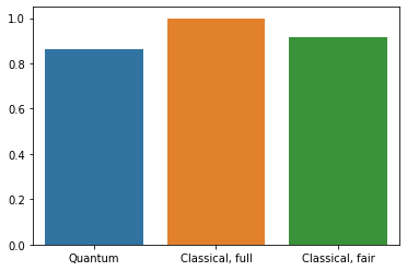
4. 比較
解像度の高い入力とより強力なモデルの場合、CNN はこの問題を簡単に解決できますが、似たようなパワー(最大 32 個のパラメータ)を持つ古典的モデルはわずかな時間で似たような精度までトレーニングすることができます。いずれにせよ、従来のニューラルネットワークは量子ニューラルネットワークの性能を簡単に上回ります。古典的なデータでは、従来のニューラルネットワークを上回るのは困難といえます。
qnn_accuracy = qnn_results[1]
cnn_accuracy = cnn_results[1]
fair_nn_accuracy = fair_nn_results[1]

sns.barplot(["Quantum", "Classical, full", "Classical, fair"],
            [qnn_accuracy, cnn_accuracy, fair_nn_accuracy])
/home/kbuilder/.local/lib/python3.6/site-packages/seaborn/_decorators.py:43: FutureWarning: Pass the following variables as keyword args: x, y. From version 0.12, the only valid positional argument will be `data`, and passing other arguments without an explicit keyword will result in an error or misinterpretation.
  FutureWarning
<AxesSubplot:>