量子畳み込みニューラルネットワーク

TensorFlow.orgで表示

Google Colab で実行

GitHub でソースを表示{

ノートブックをダウンロード/a0}

このチュートリアルでは、単純な量子畳み込みニューラルネットワーク（QCNN）を実装します。QCNN は、並進的に不変でもある古典的な畳み込みニューラルネットワークに提案された量子アナログです。

この例では、デバイスの量子センサまたは複雑なシミュレーションなど、量子データソースの特定のプロパティを検出する方法を実演します。量子データソースは、励起の有無にかかわらずクラスタ状態です。QCNN はこの検出を学習します（論文で使用されたデータセットは SPT フェーズ分類です）。

セットアップ

pip install -q tensorflow==2.3.1

TensorFlow Quantum をインストールします。

pip install -q tensorflow-quantum

次に、TensorFlow とモジュールの依存関係をインポートします。

import tensorflow as tf
import tensorflow_quantum as tfq

import cirq
import sympy
import numpy as np

# visualization tools
%matplotlib inline
import matplotlib.pyplot as plt
from cirq.contrib.svg import SVGCircuit

1. QCNN を構築する

1.1 TensorFlow グラフで回路を組み立てる

TensorFlow Quantum（TFQ）には、グラフ内で回路を構築するために設計されたレイヤークラスがあります。たとえば tfq.layers.AddCircuit レイヤーがあり、tf.keras.Layer を継承しています。このレイヤーは、次の図で示すように、回路の入力バッチの前後いずれかに追加できます。

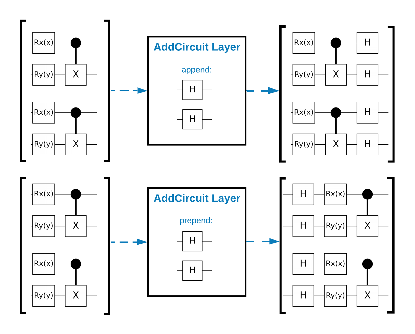
次のスニペットには、このレイヤーが使用されています。

qubit = cirq.GridQubit(0, 0)

# Define some circuits.
circuit1 = cirq.Circuit(cirq.X(qubit))
circuit2 = cirq.Circuit(cirq.H(qubit))

# Convert to a tensor.
input_circuit_tensor = tfq.convert_to_tensor([circuit1, circuit2])

# Define a circuit that we want to append
y_circuit = cirq.Circuit(cirq.Y(qubit))

# Instantiate our layer
y_appender = tfq.layers.AddCircuit()

# Run our circuit tensor through the layer and save the output.
output_circuit_tensor = y_appender(input_circuit_tensor, append=y_circuit)

入力テンソルを調べます。

print(tfq.from_tensor(input_circuit_tensor))

[cirq.Circuit([
    cirq.Moment(
        cirq.X(cirq.GridQubit(0, 0)),
    ),
])
 cirq.Circuit([
    cirq.Moment(
        cirq.H(cirq.GridQubit(0, 0)),
    ),
])]

次に、出力テンソルを調べます。

print(tfq.from_tensor(output_circuit_tensor))

[cirq.Circuit([
    cirq.Moment(
        cirq.X(cirq.GridQubit(0, 0)),
    ),
    cirq.Moment(
        cirq.Y(cirq.GridQubit(0, 0)),
    ),
])
 cirq.Circuit([
    cirq.Moment(
        cirq.H(cirq.GridQubit(0, 0)),
    ),
    cirq.Moment(
        cirq.Y(cirq.GridQubit(0, 0)),
    ),
])]

以下の例は tfq.layers.AddCircuit を使用せずに実行できますが、TensorFlow 計算グラフに複雑な機能を埋め込む方法を理解する上で役立ちます。

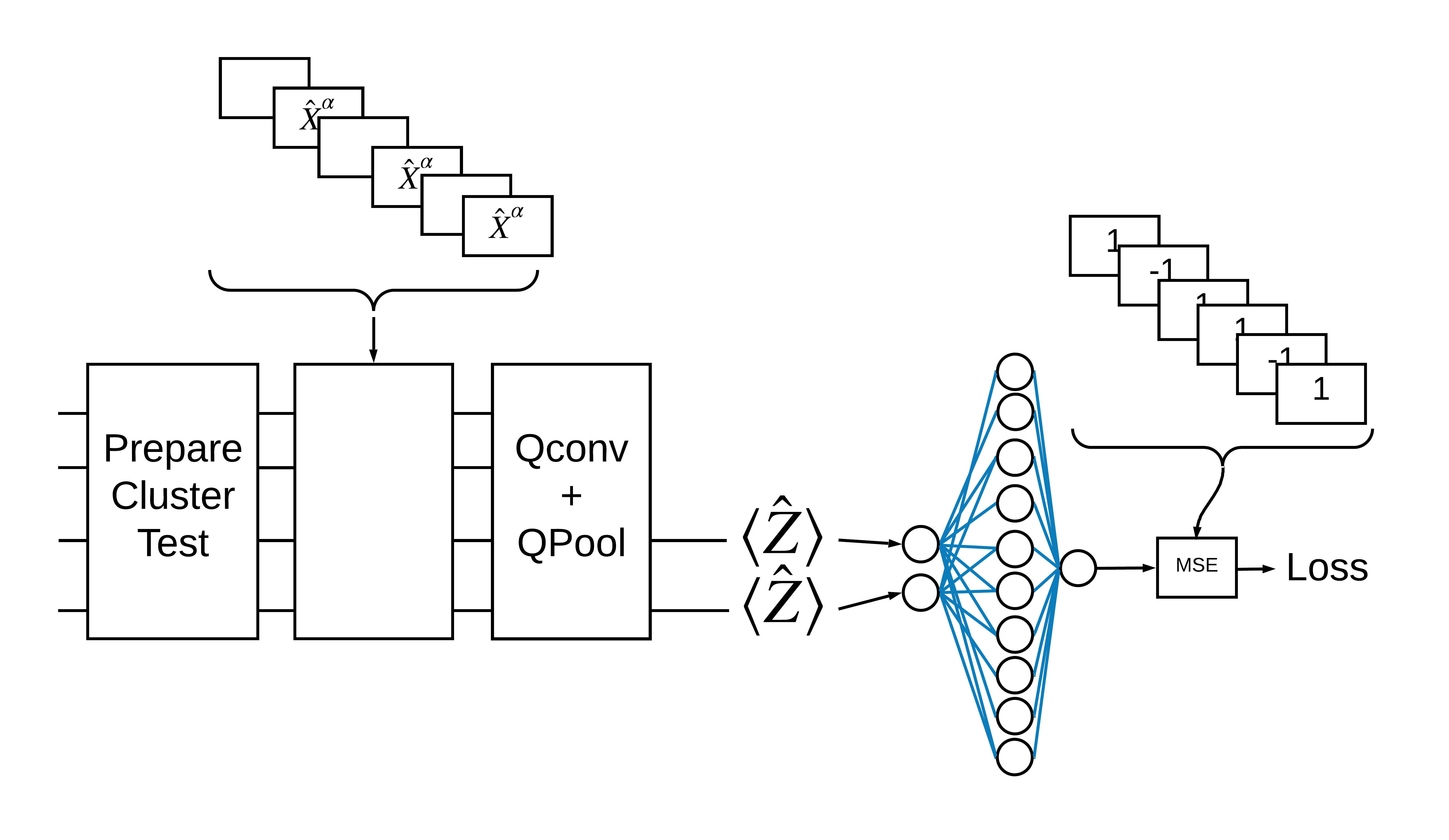
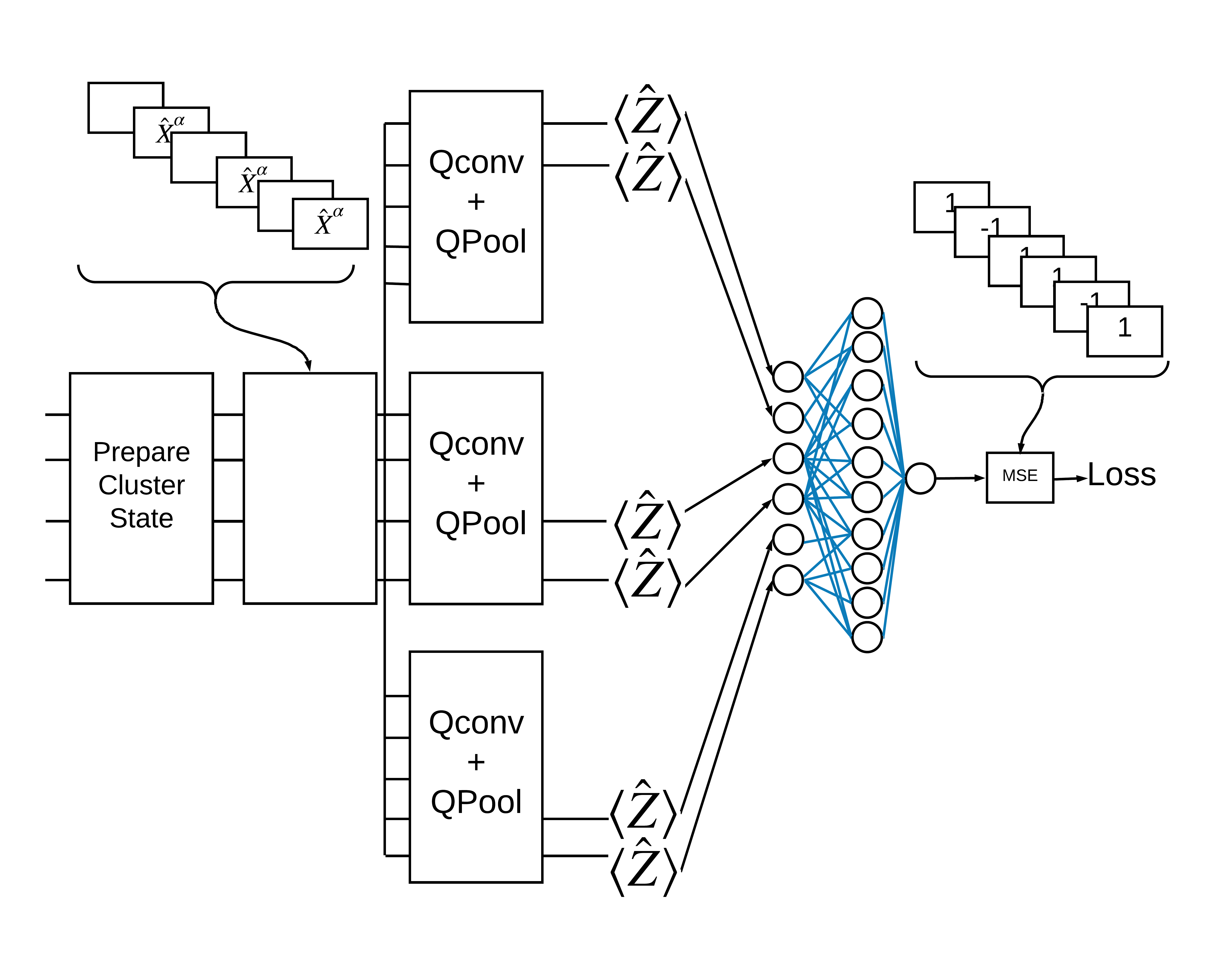
1.2 問題の概要

クラスター状態を準備し、「励起」があるかどうかを検出する量子分類器をトレーニングします。クラスター状態は極めてこじれていますが、古典的コンピュータにおいては必ずしも困難ではありません。わかりやすく言えば、これは論文で使用されているデータセットよりも単純です。

この分類タスクでは、次の理由により、ディープ MERA のような QCNN アーキテクチャを実装します。

1. QCNN と同様に、リングのクラスター状態は並進的に不変である
2. クラスター状態は非常にもつれている

このアーキテクチャはエンタングルメントを軽減し、単一のキュービットを読み出すことで分類を取得する上で効果があります。

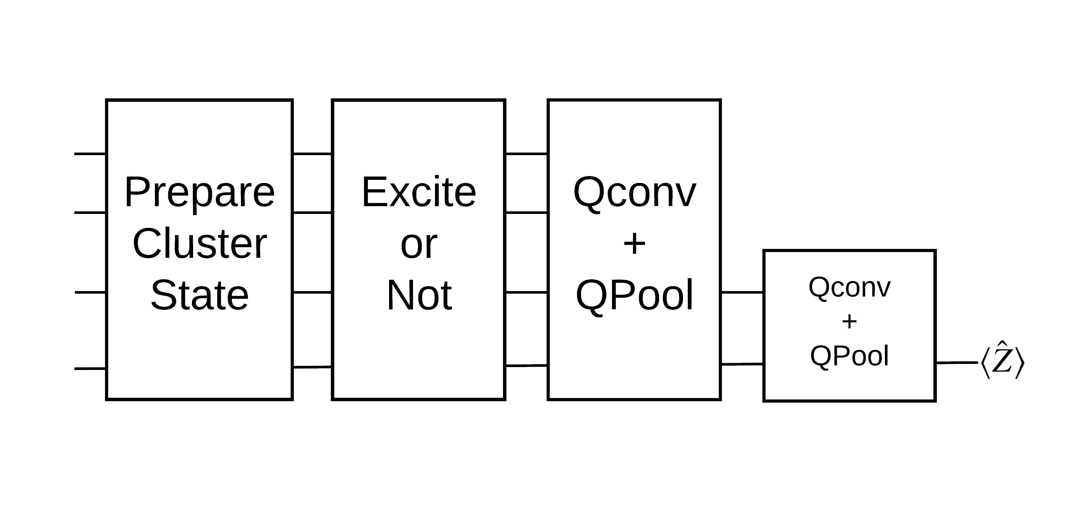
「励起」のあるクラスター状態は、cirq.rx ゲートがすべてのキュービットに適用されたクラスター状態として定義されます。Qconv と QPool については、このチュートリアルの後の方で説明しています。

1.3 TensorFlow のビルディングブロック

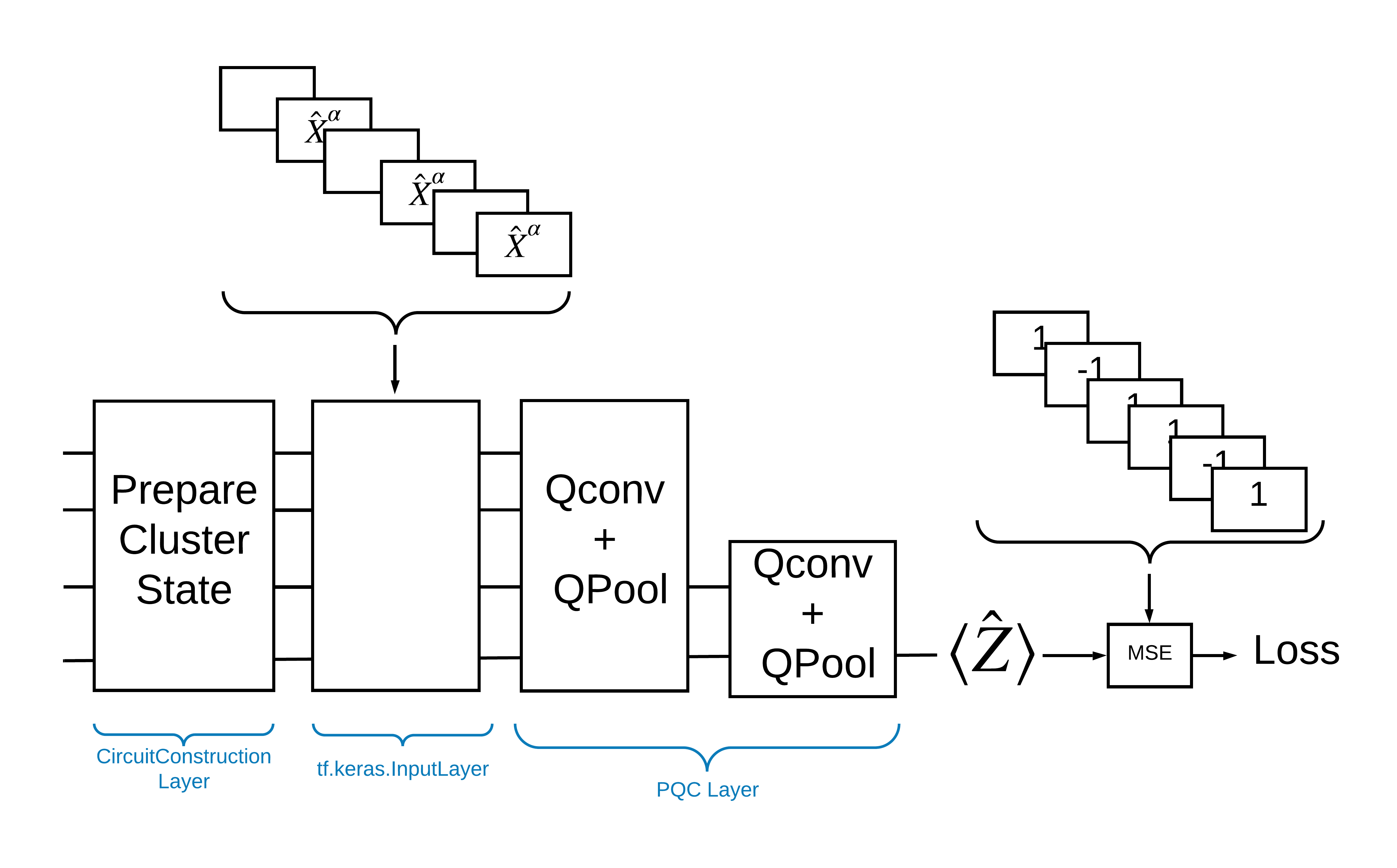
TensorFlow Quantum を使ってこの問題を解決する方法として、次を実装することが挙げられます。

1. モデルへの入力は回路で、空の回路か励起を示す特定のキュー人における X ゲートです。
2. モデルの残りの量子コンポーネントは、tfq.layers.AddCircuit レイヤーで作成されます。
3. たとえば tfq.layers.PQC レイヤーが使用されているとした場合、\(\langle \hat{Z} \rangle\) を読み取って、励起のある状態には 1 のラベルと、励起のない状態には -1 のラベルと比較します。

1.4 データ

モデルを構築する前に、データを生成することができます。この場合には、クラスター状態に励起がは一斉思案す（元の論文では、より複雑なデータセットが使用されています）。励起は、cirq.rx ゲートで表されます。十分に大きい回転は励起と見なされ、1 とラベル付けされ、十分に大きくない回転は -1 とラベル付けされ、励起ではないと見なされます。

def generate_data(qubits):
    """Generate training and testing data."""
    n_rounds = 20  # Produces n_rounds * n_qubits datapoints.
    excitations = []
    labels = []
    for n in range(n_rounds):
        for bit in qubits:
            rng = np.random.uniform(-np.pi, np.pi)
            excitations.append(cirq.Circuit(cirq.rx(rng)(bit)))
            labels.append(1 if (-np.pi / 2) <= rng <= (np.pi / 2) else -1)

    split_ind = int(len(excitations) * 0.7)
    train_excitations = excitations[:split_ind]
    test_excitations = excitations[split_ind:]

    train_labels = labels[:split_ind]
    test_labels = labels[split_ind:]

    return tfq.convert_to_tensor(train_excitations), np.array(train_labels), \
        tfq.convert_to_tensor(test_excitations), np.array(test_labels)

通常の機械学習と同じように、モデルのベンチマークに使用するトレーニングとテストのセットを作成していることがわかります。次のようにすると、データポイントを素早く確認できます。

sample_points, sample_labels, _, __ = generate_data(cirq.GridQubit.rect(1, 4))
print('Input:', tfq.from_tensor(sample_points)[0], 'Output:', sample_labels[0])
print('Input:', tfq.from_tensor(sample_points)[1], 'Output:', sample_labels[1])

Input: (0, 0): ───Rx(-0.102π)─── Output: 1
Input: (0, 1): ───Rx(-0.104π)─── Output: 1

1.5 レイヤーを定義する

上記の図で示すレイヤーを TensorFlow で定義しましょう。

1.5.1 クラスター状態

まず始めに、クラスター状態を定義しますが、これには Google が量子回路のプログラミング用に提供している Cirq フレームワークを使用します。モデルの静的な部分であるため、tfq.layers.AddCircuit 機能を使用して埋め込みます。

def cluster_state_circuit(bits):
    """Return a cluster state on the qubits in `bits`."""
    circuit = cirq.Circuit()
    circuit.append(cirq.H.on_each(bits))
    for this_bit, next_bit in zip(bits, bits[1:] + [bits[0]]):
        circuit.append(cirq.CZ(this_bit, next_bit))
    return circuit

矩形の cirq.GridQubit のクラスター状態回路を表示します。

SVGCircuit(cluster_state_circuit(cirq.GridQubit.rect(1, 4)))

findfont: Font family ['Arial'] not found. Falling back to DejaVu Sans.

1.5.2 QCNN レイヤー

Cong and Lukin の QCNN に関する論文を使用して、モデルを構成するレイヤーを定義します。これには次の前提条件があります。

• Tucci の論文にある 1 キュービットと 2 キュービットのパラメータ化されたユニタリ―行列
• 一般的なパラメータ化された 2 キュービットプーリング演算

def one_qubit_unitary(bit, symbols):
    """Make a Cirq circuit enacting a rotation of the bloch sphere about the X,
    Y and Z axis, that depends on the values in `symbols`.
    """
    return cirq.Circuit(
        cirq.X(bit)**symbols[0],
        cirq.Y(bit)**symbols[1],
        cirq.Z(bit)**symbols[2])


def two_qubit_unitary(bits, symbols):
    """Make a Cirq circuit that creates an arbitrary two qubit unitary."""
    circuit = cirq.Circuit()
    circuit += one_qubit_unitary(bits[0], symbols[0:3])
    circuit += one_qubit_unitary(bits[1], symbols[3:6])
    circuit += [cirq.ZZ(*bits)**symbols[6]]
    circuit += [cirq.YY(*bits)**symbols[7]]
    circuit += [cirq.XX(*bits)**symbols[8]]
    circuit += one_qubit_unitary(bits[0], symbols[9:12])
    circuit += one_qubit_unitary(bits[1], symbols[12:])
    return circuit


def two_qubit_pool(source_qubit, sink_qubit, symbols):
    """Make a Cirq circuit to do a parameterized 'pooling' operation, which
    attempts to reduce entanglement down from two qubits to just one."""
    pool_circuit = cirq.Circuit()
    sink_basis_selector = one_qubit_unitary(sink_qubit, symbols[0:3])
    source_basis_selector = one_qubit_unitary(source_qubit, symbols[3:6])
    pool_circuit.append(sink_basis_selector)
    pool_circuit.append(source_basis_selector)
    pool_circuit.append(cirq.CNOT(control=source_qubit, target=sink_qubit))
    pool_circuit.append(sink_basis_selector**-1)
    return pool_circuit

作成したものを確認するために、1 キュービットのユニタリー回路を出力しましょう。

SVGCircuit(one_qubit_unitary(cirq.GridQubit(0, 0), sympy.symbols('x0:3')))

次に、2 キュービットのユニタリー回路を出力します。

SVGCircuit(two_qubit_unitary(cirq.GridQubit.rect(1, 2), sympy.symbols('x0:15')))

そして 2 キュービットのプーリング回路を出力します。

SVGCircuit(two_qubit_pool(*cirq.GridQubit.rect(1, 2), sympy.symbols('x0:6')))

1.5.2.1 量子畳み込み

Cong と Lukin の論文にあるとおり、1 次元量子畳み込みを、ストライド 1 の隣接するすべてのキュービットペアに 2 キュービットのパラメーター化されたユニタリの適用として定義します。

def quantum_conv_circuit(bits, symbols):
    """Quantum Convolution Layer following the above diagram.
    Return a Cirq circuit with the cascade of `two_qubit_unitary` applied
    to all pairs of qubits in `bits` as in the diagram above.
    """
    circuit = cirq.Circuit()
    for first, second in zip(bits[0::2], bits[1::2]):
        circuit += two_qubit_unitary([first, second], symbols)
    for first, second in zip(bits[1::2], bits[2::2] + [bits[0]]):
        circuit += two_qubit_unitary([first, second], symbols)
    return circuit

（非常に水平な）回路を表示します。

SVGCircuit(
    quantum_conv_circuit(cirq.GridQubit.rect(1, 8), sympy.symbols('x0:15')))

1.5.2.2 量子プーリング

量子プーリングレイヤーは、上記で定義された 2 キュービットプールを使用して、\(N\) キュービットから \(\frac{N}{2}\) キュービットまでをプーリングします。

def quantum_pool_circuit(source_bits, sink_bits, symbols):
    """A layer that specifies a quantum pooling operation.
    A Quantum pool tries to learn to pool the relevant information from two
    qubits onto 1.
    """
    circuit = cirq.Circuit()
    for source, sink in zip(source_bits, sink_bits):
        circuit += two_qubit_pool(source, sink, symbols)
    return circuit

プーリングコンポーネント回路を調べます。

test_bits = cirq.GridQubit.rect(1, 8)

SVGCircuit(
    quantum_pool_circuit(test_bits[:4], test_bits[4:], sympy.symbols('x0:6')))

1.6 モデルの定義

定義したレイヤーを使用して純粋な量子 CNN を構築します。8 キュービットで開始し、1 キュービットまでプールダウンしてから、\(\langle \hat{Z} \rangle\) を測定します。

def create_model_circuit(qubits):
    """Create sequence of alternating convolution and pooling operators 
    which gradually shrink over time."""
    model_circuit = cirq.Circuit()
    symbols = sympy.symbols('qconv0:63')
    # Cirq uses sympy.Symbols to map learnable variables. TensorFlow Quantum
    # scans incoming circuits and replaces these with TensorFlow variables.
    model_circuit += quantum_conv_circuit(qubits, symbols[0:15])
    model_circuit += quantum_pool_circuit(qubits[:4], qubits[4:],
                                          symbols[15:21])
    model_circuit += quantum_conv_circuit(qubits[4:], symbols[21:36])
    model_circuit += quantum_pool_circuit(qubits[4:6], qubits[6:],
                                          symbols[36:42])
    model_circuit += quantum_conv_circuit(qubits[6:], symbols[42:57])
    model_circuit += quantum_pool_circuit([qubits[6]], [qubits[7]],
                                          symbols[57:63])
    return model_circuit


# Create our qubits and readout operators in Cirq.
cluster_state_bits = cirq.GridQubit.rect(1, 8)
readout_operators = cirq.Z(cluster_state_bits[-1])

# Build a sequential model enacting the logic in 1.3 of this notebook.
# Here you are making the static cluster state prep as a part of the AddCircuit and the
# "quantum datapoints" are coming in the form of excitation
excitation_input = tf.keras.Input(shape=(), dtype=tf.dtypes.string)
cluster_state = tfq.layers.AddCircuit()(
    excitation_input, prepend=cluster_state_circuit(cluster_state_bits))

quantum_model = tfq.layers.PQC(create_model_circuit(cluster_state_bits),
                               readout_operators)(cluster_state)

qcnn_model = tf.keras.Model(inputs=[excitation_input], outputs=[quantum_model])

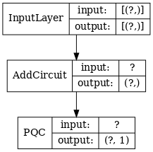
# Show the keras plot of the model
tf.keras.utils.plot_model(qcnn_model,
                          show_shapes=True,
                          show_layer_names=False,
                          dpi=70)

1.7 モデルをトレーニングする

この例を単純化するために、完全なバッチでモデルをトレーニングします。

# Generate some training data.
train_excitations, train_labels, test_excitations, test_labels = generate_data(
    cluster_state_bits)


# Custom accuracy metric.
@tf.function
def custom_accuracy(y_true, y_pred):
    y_true = tf.squeeze(y_true)
    y_pred = tf.map_fn(lambda x: 1.0 if x >= 0 else -1.0, y_pred)
    return tf.keras.backend.mean(tf.keras.backend.equal(y_true, y_pred))


qcnn_model.compile(optimizer=tf.keras.optimizers.Adam(learning_rate=0.02),
                   loss=tf.losses.mse,
                   metrics=[custom_accuracy])

history = qcnn_model.fit(x=train_excitations,
                         y=train_labels,
                         batch_size=16,
                         epochs=25,
                         verbose=1,
                         validation_data=(test_excitations, test_labels))

Epoch 1/25
7/7 [==============================] - 1s 128ms/step - loss: 0.8843 - custom_accuracy: 0.6964 - val_loss: 0.7839 - val_custom_accuracy: 0.7083
Epoch 2/25
7/7 [==============================] - 1s 102ms/step - loss: 0.7946 - custom_accuracy: 0.7411 - val_loss: 0.7767 - val_custom_accuracy: 0.7708
Epoch 3/25
7/7 [==============================] - 1s 99ms/step - loss: 0.7505 - custom_accuracy: 0.7500 - val_loss: 0.7514 - val_custom_accuracy: 0.6458
Epoch 4/25
7/7 [==============================] - 1s 96ms/step - loss: 0.7281 - custom_accuracy: 0.7589 - val_loss: 0.7199 - val_custom_accuracy: 0.8125
Epoch 5/25
7/7 [==============================] - 1s 96ms/step - loss: 0.7121 - custom_accuracy: 0.7946 - val_loss: 0.7120 - val_custom_accuracy: 0.8125
Epoch 6/25
7/7 [==============================] - 1s 97ms/step - loss: 0.7066 - custom_accuracy: 0.8214 - val_loss: 0.7182 - val_custom_accuracy: 0.8125
Epoch 7/25
7/7 [==============================] - 1s 94ms/step - loss: 0.6944 - custom_accuracy: 0.8393 - val_loss: 0.7058 - val_custom_accuracy: 0.8750
Epoch 8/25
7/7 [==============================] - 1s 94ms/step - loss: 0.6940 - custom_accuracy: 0.8571 - val_loss: 0.7340 - val_custom_accuracy: 0.7708
Epoch 9/25
7/7 [==============================] - 1s 95ms/step - loss: 0.6838 - custom_accuracy: 0.8929 - val_loss: 0.6876 - val_custom_accuracy: 0.8542
Epoch 10/25
7/7 [==============================] - 1s 94ms/step - loss: 0.6459 - custom_accuracy: 0.8839 - val_loss: 0.6538 - val_custom_accuracy: 0.8125
Epoch 11/25
7/7 [==============================] - 1s 95ms/step - loss: 0.5875 - custom_accuracy: 0.8750 - val_loss: 0.6134 - val_custom_accuracy: 0.8125
Epoch 12/25
7/7 [==============================] - 1s 92ms/step - loss: 0.5375 - custom_accuracy: 0.8125 - val_loss: 0.5855 - val_custom_accuracy: 0.6667
Epoch 13/25
7/7 [==============================] - 1s 89ms/step - loss: 0.5062 - custom_accuracy: 0.8036 - val_loss: 0.5798 - val_custom_accuracy: 0.7083
Epoch 14/25
7/7 [==============================] - 1s 89ms/step - loss: 0.5071 - custom_accuracy: 0.8304 - val_loss: 0.5781 - val_custom_accuracy: 0.7292
Epoch 15/25
7/7 [==============================] - 1s 91ms/step - loss: 0.5062 - custom_accuracy: 0.8036 - val_loss: 0.5772 - val_custom_accuracy: 0.6875
Epoch 16/25
7/7 [==============================] - 1s 91ms/step - loss: 0.5037 - custom_accuracy: 0.7857 - val_loss: 0.5751 - val_custom_accuracy: 0.6875
Epoch 17/25
7/7 [==============================] - 1s 91ms/step - loss: 0.4947 - custom_accuracy: 0.7768 - val_loss: 0.5747 - val_custom_accuracy: 0.7083
Epoch 18/25
7/7 [==============================] - 1s 90ms/step - loss: 0.4875 - custom_accuracy: 0.7768 - val_loss: 0.5717 - val_custom_accuracy: 0.6667
Epoch 19/25
7/7 [==============================] - 1s 92ms/step - loss: 0.5015 - custom_accuracy: 0.8125 - val_loss: 0.5885 - val_custom_accuracy: 0.7292
Epoch 20/25
7/7 [==============================] - 1s 90ms/step - loss: 0.4941 - custom_accuracy: 0.8036 - val_loss: 0.5765 - val_custom_accuracy: 0.6875
Epoch 21/25
7/7 [==============================] - 1s 90ms/step - loss: 0.4830 - custom_accuracy: 0.8036 - val_loss: 0.5753 - val_custom_accuracy: 0.7500
Epoch 22/25
7/7 [==============================] - 1s 88ms/step - loss: 0.4861 - custom_accuracy: 0.8125 - val_loss: 0.5649 - val_custom_accuracy: 0.7292
Epoch 23/25
7/7 [==============================] - 1s 89ms/step - loss: 0.4845 - custom_accuracy: 0.8304 - val_loss: 0.5788 - val_custom_accuracy: 0.7292
Epoch 24/25
7/7 [==============================] - 1s 93ms/step - loss: 0.5024 - custom_accuracy: 0.7946 - val_loss: 0.5973 - val_custom_accuracy: 0.6667
Epoch 25/25
7/7 [==============================] - 1s 90ms/step - loss: 0.5012 - custom_accuracy: 0.8036 - val_loss: 0.5942 - val_custom_accuracy: 0.7500

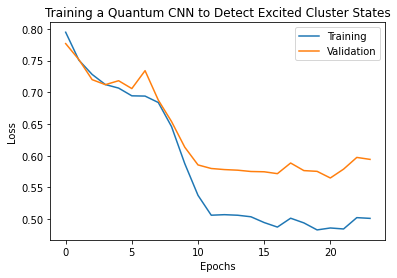
plt.plot(history.history['loss'][1:], label='Training')
plt.plot(history.history['val_loss'][1:], label='Validation')
plt.title('Training a Quantum CNN to Detect Excited Cluster States')
plt.xlabel('Epochs')
plt.ylabel('Loss')
plt.legend()
plt.show()

2. ハイブリッドモデル

量子畳み込みを使用して 8 キュービットから 1 キュービットにする必要はありません。量子畳み込みの 1～2 ラウンドを実行し、結果を従来のニューラルネットワークにフィードすることも可能です。このセクションでは、量子と従来のハイブリッドモデルを説明します。

2.1 単一量子フィルタを備えたハイブリッドモデル

量子畳み込みのレイヤーを 1 つ適用し、すべてのビットの \(\langle \hat{Z}_n \rangle\) を読み取り、続いて密に接続されたニューラルネットワークを読み取ります。

2.1.1 モデルの定義

# 1-local operators to read out
readouts = [cirq.Z(bit) for bit in cluster_state_bits[4:]]


def multi_readout_model_circuit(qubits):
    """Make a model circuit with less quantum pool and conv operations."""
    model_circuit = cirq.Circuit()
    symbols = sympy.symbols('qconv0:21')
    model_circuit += quantum_conv_circuit(qubits, symbols[0:15])
    model_circuit += quantum_pool_circuit(qubits[:4], qubits[4:],
                                          symbols[15:21])
    return model_circuit


# Build a model enacting the logic in 2.1 of this notebook.
excitation_input_dual = tf.keras.Input(shape=(), dtype=tf.dtypes.string)

cluster_state_dual = tfq.layers.AddCircuit()(
    excitation_input_dual, prepend=cluster_state_circuit(cluster_state_bits))

quantum_model_dual = tfq.layers.PQC(
    multi_readout_model_circuit(cluster_state_bits),
    readouts)(cluster_state_dual)

d1_dual = tf.keras.layers.Dense(8)(quantum_model_dual)

d2_dual = tf.keras.layers.Dense(1)(d1_dual)

hybrid_model = tf.keras.Model(inputs=[excitation_input_dual], outputs=[d2_dual])

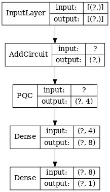
# Display the model architecture
tf.keras.utils.plot_model(hybrid_model,
                          show_shapes=True,
                          show_layer_names=False,
                          dpi=70)

2.1.2 モデルをトレーニングする

hybrid_model.compile(optimizer=tf.keras.optimizers.Adam(learning_rate=0.02),
                     loss=tf.losses.mse,
                     metrics=[custom_accuracy])

hybrid_history = hybrid_model.fit(x=train_excitations,
                                  y=train_labels,
                                  batch_size=16,
                                  epochs=25,
                                  verbose=1,
                                  validation_data=(test_excitations,
                                                   test_labels))

Epoch 1/25
7/7 [==============================] - 1s 77ms/step - loss: 0.8001 - custom_accuracy: 0.7054 - val_loss: 0.3556 - val_custom_accuracy: 0.9375
Epoch 2/25
7/7 [==============================] - 0s 57ms/step - loss: 0.3298 - custom_accuracy: 0.9286 - val_loss: 0.2516 - val_custom_accuracy: 0.9375
Epoch 3/25
7/7 [==============================] - 0s 57ms/step - loss: 0.2807 - custom_accuracy: 0.9554 - val_loss: 0.2546 - val_custom_accuracy: 0.9792
Epoch 4/25
7/7 [==============================] - 0s 57ms/step - loss: 0.2420 - custom_accuracy: 0.9821 - val_loss: 0.1967 - val_custom_accuracy: 0.9792
Epoch 5/25
7/7 [==============================] - 0s 59ms/step - loss: 0.2088 - custom_accuracy: 1.0000 - val_loss: 0.1852 - val_custom_accuracy: 0.9792
Epoch 6/25
7/7 [==============================] - 0s 59ms/step - loss: 0.2045 - custom_accuracy: 0.9911 - val_loss: 0.1840 - val_custom_accuracy: 0.9792
Epoch 7/25
7/7 [==============================] - 0s 57ms/step - loss: 0.2087 - custom_accuracy: 0.9554 - val_loss: 0.1889 - val_custom_accuracy: 0.9792
Epoch 8/25
7/7 [==============================] - 0s 55ms/step - loss: 0.2055 - custom_accuracy: 0.9821 - val_loss: 0.1970 - val_custom_accuracy: 1.0000
Epoch 9/25
7/7 [==============================] - 0s 55ms/step - loss: 0.2078 - custom_accuracy: 0.9911 - val_loss: 0.1835 - val_custom_accuracy: 1.0000
Epoch 10/25
7/7 [==============================] - 0s 57ms/step - loss: 0.1962 - custom_accuracy: 0.9911 - val_loss: 0.1787 - val_custom_accuracy: 1.0000
Epoch 11/25
7/7 [==============================] - 0s 56ms/step - loss: 0.1884 - custom_accuracy: 0.9911 - val_loss: 0.1884 - val_custom_accuracy: 1.0000
Epoch 12/25
7/7 [==============================] - 0s 55ms/step - loss: 0.1871 - custom_accuracy: 1.0000 - val_loss: 0.1869 - val_custom_accuracy: 1.0000
Epoch 13/25
7/7 [==============================] - 0s 59ms/step - loss: 0.1854 - custom_accuracy: 1.0000 - val_loss: 0.1799 - val_custom_accuracy: 1.0000
Epoch 14/25
7/7 [==============================] - 0s 58ms/step - loss: 0.1881 - custom_accuracy: 1.0000 - val_loss: 0.1824 - val_custom_accuracy: 1.0000
Epoch 15/25
7/7 [==============================] - 0s 58ms/step - loss: 0.1965 - custom_accuracy: 0.9821 - val_loss: 0.1733 - val_custom_accuracy: 1.0000
Epoch 16/25
7/7 [==============================] - 0s 56ms/step - loss: 0.1884 - custom_accuracy: 1.0000 - val_loss: 0.1768 - val_custom_accuracy: 1.0000
Epoch 17/25
7/7 [==============================] - 0s 58ms/step - loss: 0.1948 - custom_accuracy: 0.9732 - val_loss: 0.1831 - val_custom_accuracy: 1.0000
Epoch 18/25
7/7 [==============================] - 0s 58ms/step - loss: 0.1937 - custom_accuracy: 0.9732 - val_loss: 0.1869 - val_custom_accuracy: 1.0000
Epoch 19/25
7/7 [==============================] - 0s 59ms/step - loss: 0.1928 - custom_accuracy: 0.9732 - val_loss: 0.1818 - val_custom_accuracy: 1.0000
Epoch 20/25
7/7 [==============================] - 0s 59ms/step - loss: 0.1878 - custom_accuracy: 1.0000 - val_loss: 0.1687 - val_custom_accuracy: 1.0000
Epoch 21/25
7/7 [==============================] - 0s 61ms/step - loss: 0.1884 - custom_accuracy: 1.0000 - val_loss: 0.1760 - val_custom_accuracy: 1.0000
Epoch 22/25
7/7 [==============================] - 0s 59ms/step - loss: 0.1809 - custom_accuracy: 0.9821 - val_loss: 0.1965 - val_custom_accuracy: 1.0000
Epoch 23/25
7/7 [==============================] - 0s 59ms/step - loss: 0.1880 - custom_accuracy: 0.9911 - val_loss: 0.1738 - val_custom_accuracy: 1.0000
Epoch 24/25
7/7 [==============================] - 0s 59ms/step - loss: 0.1901 - custom_accuracy: 1.0000 - val_loss: 0.1879 - val_custom_accuracy: 1.0000
Epoch 25/25
7/7 [==============================] - 0s 59ms/step - loss: 0.1874 - custom_accuracy: 0.9821 - val_loss: 0.1845 - val_custom_accuracy: 1.0000

plt.plot(history.history['val_custom_accuracy'], label='QCNN')
plt.plot(hybrid_history.history['val_custom_accuracy'], label='Hybrid CNN')
plt.title('Quantum vs Hybrid CNN performance')
plt.xlabel('Epochs')
plt.legend()
plt.ylabel('Validation Accuracy')
plt.show()

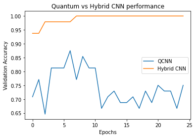
ご覧のとおり、非常に控えめな古典的支援により、ハイブリッドモデルは通常、純粋な量子バージョンよりも速く収束します。

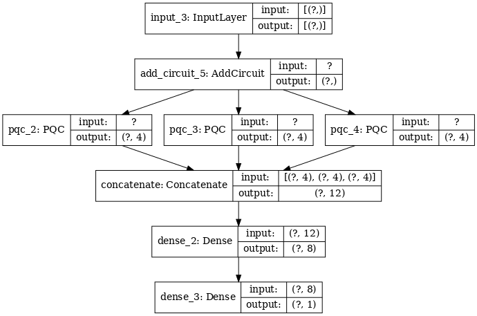
2.2 多重量子フィルタを備えたハイブリッド畳み込み

多重量子畳み込みと従来のニューラルネットワークを使用してそれらを組み合わせるアーキテクチャを試してみましょう。

2.2.1 モデルの定義

excitation_input_multi = tf.keras.Input(shape=(), dtype=tf.dtypes.string)

cluster_state_multi = tfq.layers.AddCircuit()(
    excitation_input_multi, prepend=cluster_state_circuit(cluster_state_bits))

# apply 3 different filters and measure expectation values

quantum_model_multi1 = tfq.layers.PQC(
    multi_readout_model_circuit(cluster_state_bits),
    readouts)(cluster_state_multi)

quantum_model_multi2 = tfq.layers.PQC(
    multi_readout_model_circuit(cluster_state_bits),
    readouts)(cluster_state_multi)

quantum_model_multi3 = tfq.layers.PQC(
    multi_readout_model_circuit(cluster_state_bits),
    readouts)(cluster_state_multi)

# concatenate outputs and feed into a small classical NN
concat_out = tf.keras.layers.concatenate(
    [quantum_model_multi1, quantum_model_multi2, quantum_model_multi3])

dense_1 = tf.keras.layers.Dense(8)(concat_out)

dense_2 = tf.keras.layers.Dense(1)(dense_1)

multi_qconv_model = tf.keras.Model(inputs=[excitation_input_multi],
                                   outputs=[dense_2])

# Display the model architecture
tf.keras.utils.plot_model(multi_qconv_model,
                          show_shapes=True,
                          show_layer_names=True,
                          dpi=70)

2.2.2 モデルをトレーニングする

multi_qconv_model.compile(
    optimizer=tf.keras.optimizers.Adam(learning_rate=0.02),
    loss=tf.losses.mse,
    metrics=[custom_accuracy])

multi_qconv_history = multi_qconv_model.fit(x=train_excitations,
                                            y=train_labels,
                                            batch_size=16,
                                            epochs=25,
                                            verbose=1,
                                            validation_data=(test_excitations,
                                                             test_labels))

Epoch 1/25
7/7 [==============================] - 1s 110ms/step - loss: 0.7519 - custom_accuracy: 0.7679 - val_loss: 0.5226 - val_custom_accuracy: 0.8750
Epoch 2/25
7/7 [==============================] - 1s 84ms/step - loss: 0.3448 - custom_accuracy: 0.9286 - val_loss: 0.2624 - val_custom_accuracy: 0.9792
Epoch 3/25
7/7 [==============================] - 1s 84ms/step - loss: 0.2618 - custom_accuracy: 0.9375 - val_loss: 0.2998 - val_custom_accuracy: 0.9375
Epoch 4/25
7/7 [==============================] - 1s 83ms/step - loss: 0.2450 - custom_accuracy: 0.9732 - val_loss: 0.2298 - val_custom_accuracy: 0.9792
Epoch 5/25
7/7 [==============================] - 1s 77ms/step - loss: 0.2133 - custom_accuracy: 0.9554 - val_loss: 0.2444 - val_custom_accuracy: 0.9375
Epoch 6/25
7/7 [==============================] - 1s 79ms/step - loss: 0.2018 - custom_accuracy: 0.9643 - val_loss: 0.2128 - val_custom_accuracy: 0.9792
Epoch 7/25
7/7 [==============================] - 1s 88ms/step - loss: 0.1994 - custom_accuracy: 0.9821 - val_loss: 0.1889 - val_custom_accuracy: 0.9583
Epoch 8/25
7/7 [==============================] - 1s 82ms/step - loss: 0.2024 - custom_accuracy: 0.9732 - val_loss: 0.2196 - val_custom_accuracy: 0.9583
Epoch 9/25
7/7 [==============================] - 1s 82ms/step - loss: 0.1967 - custom_accuracy: 0.9732 - val_loss: 0.2129 - val_custom_accuracy: 1.0000
Epoch 10/25
7/7 [==============================] - 1s 80ms/step - loss: 0.1952 - custom_accuracy: 0.9732 - val_loss: 0.1964 - val_custom_accuracy: 1.0000
Epoch 11/25
7/7 [==============================] - 1s 81ms/step - loss: 0.1945 - custom_accuracy: 0.9821 - val_loss: 0.1918 - val_custom_accuracy: 0.9792
Epoch 12/25
7/7 [==============================] - 1s 79ms/step - loss: 0.1890 - custom_accuracy: 0.9821 - val_loss: 0.2117 - val_custom_accuracy: 0.9583
Epoch 13/25
7/7 [==============================] - 1s 81ms/step - loss: 0.1891 - custom_accuracy: 0.9821 - val_loss: 0.2201 - val_custom_accuracy: 0.9375
Epoch 14/25
7/7 [==============================] - 1s 84ms/step - loss: 0.1936 - custom_accuracy: 0.9821 - val_loss: 0.2184 - val_custom_accuracy: 0.9792
Epoch 15/25
7/7 [==============================] - 1s 82ms/step - loss: 0.2028 - custom_accuracy: 0.9821 - val_loss: 0.2323 - val_custom_accuracy: 0.9792
Epoch 16/25
7/7 [==============================] - 1s 79ms/step - loss: 0.2221 - custom_accuracy: 0.9732 - val_loss: 0.2088 - val_custom_accuracy: 0.9792
Epoch 17/25
7/7 [==============================] - 1s 83ms/step - loss: 0.2225 - custom_accuracy: 0.9554 - val_loss: 0.1994 - val_custom_accuracy: 0.9583
Epoch 18/25
7/7 [==============================] - 1s 83ms/step - loss: 0.1849 - custom_accuracy: 0.9732 - val_loss: 0.1880 - val_custom_accuracy: 0.9792
Epoch 19/25
7/7 [==============================] - 1s 82ms/step - loss: 0.1919 - custom_accuracy: 0.9821 - val_loss: 0.1857 - val_custom_accuracy: 1.0000
Epoch 20/25
7/7 [==============================] - 1s 79ms/step - loss: 0.1907 - custom_accuracy: 0.9821 - val_loss: 0.2216 - val_custom_accuracy: 0.9792
Epoch 21/25
7/7 [==============================] - 1s 82ms/step - loss: 0.1929 - custom_accuracy: 0.9821 - val_loss: 0.1753 - val_custom_accuracy: 1.0000
Epoch 22/25
7/7 [==============================] - 1s 89ms/step - loss: 0.1903 - custom_accuracy: 0.9821 - val_loss: 0.1792 - val_custom_accuracy: 1.0000
Epoch 23/25
7/7 [==============================] - 1s 84ms/step - loss: 0.1875 - custom_accuracy: 0.9821 - val_loss: 0.1998 - val_custom_accuracy: 1.0000
Epoch 24/25
7/7 [==============================] - 1s 86ms/step - loss: 0.1884 - custom_accuracy: 0.9643 - val_loss: 0.2063 - val_custom_accuracy: 1.0000
Epoch 25/25
7/7 [==============================] - 1s 81ms/step - loss: 0.1945 - custom_accuracy: 0.9821 - val_loss: 0.1902 - val_custom_accuracy: 1.0000

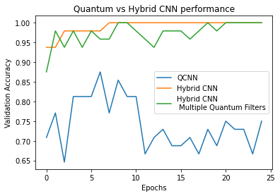
plt.plot(history.history['val_custom_accuracy'][:25], label='QCNN')
plt.plot(hybrid_history.history['val_custom_accuracy'][:25], label='Hybrid CNN')
plt.plot(multi_qconv_history.history['val_custom_accuracy'][:25],
         label='Hybrid CNN \n Multiple Quantum Filters')
plt.title('Quantum vs Hybrid CNN performance')
plt.xlabel('Epochs')
plt.legend()
plt.ylabel('Validation Accuracy')
plt.show()