
| | |  Wyświetl źródło na GitHub Wyświetl źródło na GitHub | |
Ten poradnik klasyfikacja tekst trenuje nawracające sieci neuronowej na IMDB duży filmowego przeglądu zbioru danych do analizy nastrojów.
Ustawiać
import numpy as np

import tensorflow_datasets as tfds
import tensorflow as tf

tfds.disable_progress_bar()
Import matplotlib i utworzyć funkcję pomocnika do wykresów działki:
import matplotlib.pyplot as plt


def plot_graphs(history, metric):
  plt.plot(history.history[metric])
  plt.plot(history.history['val_'+metric], '')
  plt.xlabel("Epochs")
  plt.ylabel(metric)
  plt.legend([metric, 'val_'+metric])
Konfiguracja potoku wejściowego
IMDb duży przegląd filmowy zbiór danych jest binarny klasyfikacji zbioru danych-wszystkie opinie mają zarówno pozytywny lub negatywny sentyment.
Pobierz zestaw danych za pomocą TFDS . Zobacz poradnik tekstowy ładowania Szczegółowe informacje na temat ładowania tego rodzaju danych ręcznie.
dataset, info = tfds.load('imdb_reviews', with_info=True,
                          as_supervised=True)
train_dataset, test_dataset = dataset['train'], dataset['test']

train_dataset.element_spec
(TensorSpec(shape=(), dtype=tf.string, name=None),
 TensorSpec(shape=(), dtype=tf.int64, name=None))
Początkowo zwraca zestaw danych (tekst, pary etykiet):
for example, label in train_dataset.take(1):
  print('text: ', example.numpy())
  print('label: ', label.numpy())
text:  b"This was an absolutely terrible movie. Don't be lured in by Christopher Walken or Michael Ironside. Both are great actors, but this must simply be their worst role in history. Even their great acting could not redeem this movie's ridiculous storyline. This movie is an early nineties US propaganda piece. The most pathetic scenes were those when the Columbian rebels were making their cases for revolutions. Maria Conchita Alonso appeared phony, and her pseudo-love affair with Walken was nothing but a pathetic emotional plug in a movie that was devoid of any real meaning. I am disappointed that there are movies like this, ruining actor's like Christopher Walken's good name. I could barely sit through it."
label:  0
Następny losowe dane dotyczące szkolenia i tworzenia partii tych (text, label) w parach:
BUFFER_SIZE = 10000
BATCH_SIZE = 64
train_dataset = train_dataset.shuffle(BUFFER_SIZE).batch(BATCH_SIZE).prefetch(tf.data.AUTOTUNE)
test_dataset = test_dataset.batch(BATCH_SIZE).prefetch(tf.data.AUTOTUNE)
for example, label in train_dataset.take(1):
  print('texts: ', example.numpy()[:3])
  print()
  print('labels: ', label.numpy()[:3])
texts:  [b'This is arguably the worst film I have ever seen, and I have quite an appetite for awful (and good) movies. It could (just) have managed a kind of adolescent humour if it had been consistently tongue-in-cheek --\xc3\xa0 la ROCKY HORROR PICTURE SHOW, which was really very funny. Other movies, like PLAN NINE FROM OUTER SPACE, manage to be funny while (apparently) trying to be serious. As to the acting, it looks like they rounded up brain-dead teenagers and asked them to ad-lib the whole production. Compared to them, Tom Cruise looks like Alec Guinness. There was one decent interpretation -- that of the older ghoul-busting broad on the motorcycle.'
 b"I saw this film in the worst possible circumstance. I'd already missed 15 minutes when I woke up to it on an international flight between Sydney and Seoul. I didn't know what I was watching, I thought maybe it was a movie of the week, but quickly became riveted by the performance of the lead actress playing a young woman who's child had been kidnapped. The premise started taking twist and turns I didn't see coming and by the end credits I was scrambling through the the in-flight guide to figure out what I had just watched. Turns out I was belatedly discovering Do-yeon Jeon who'd won Best Actress at Cannes for the role. I don't know if Secret Sunshine is typical of Korean cinema but I'm off to the DVD store to discover more."
 b"Hello. I am Paul Raddick, a.k.a. Panic Attack of WTAF, Channel 29 in Philadelphia. Let me tell you about this god awful movie that powered on Adam Sandler's film career but was digitized after a short time.<br /><br />Going Overboard is about an aspiring comedian played by Sandler who gets a job on a cruise ship and fails...or so I thought. Sandler encounters babes that like History of the World Part 1 and Rebound. The babes were supposed to be engaged, but, actually, they get executed by Sawtooth, the meanest cannibal the world has ever known. Adam Sandler fared bad in Going Overboard, but fared better in Big Daddy, Billy Madison, and Jen Leone's favorite, 50 First Dates. Man, Drew Barrymore was one hot chick. Spanglish is red hot, Going Overboard ain't Dooley squat! End of file."]

labels:  [0 1 0]
Utwórz koder tekstu
Tekst surowy ładowane tfds musi zostać przetworzony przed może być stosowany w modelu. Najprostszym sposobem na tekście procesu szkolenia używa TextVectorization warstwę. Ta warstwa ma wiele możliwości, ale ten samouczek trzyma się domyślnego zachowania.
Tworzenie warstwy, i przekazać tekst danej jednostki do warstwy .adapt metody:
VOCAB_SIZE = 1000
encoder = tf.keras.layers.TextVectorization(
    max_tokens=VOCAB_SIZE)
encoder.adapt(train_dataset.map(lambda text, label: text))
.adapt metoda ustawia słownictwa warstwy. Oto pierwsze 20 tokenów. Po uzupełnieniu i nieznanych tokenach są one sortowane według częstotliwości:
vocab = np.array(encoder.get_vocabulary())
vocab[:20]
array(['', '[UNK]', 'the', 'and', 'a', 'of', 'to', 'is', 'in', 'it', 'i',
       'this', 'that', 'br', 'was', 'as', 'for', 'with', 'movie', 'but'],
      dtype='<U14')
Po ustawieniu słownika warstwa może kodować tekst w indeksy. W tensory indeksów są 0-usztywniane najdłuższej sekwencji w partii (chyba ustawić stałą output_sequence_length ):
encoded_example = encoder(example)[:3].numpy()
encoded_example
array([[ 11,   7,   1, ...,   0,   0,   0],
       [ 10, 208,  11, ...,   0,   0,   0],
       [  1,  10, 237, ...,   0,   0,   0]])
Przy ustawieniach domyślnych proces nie jest całkowicie odwracalny. Istnieją trzy główne powody:
- Domyślna wartość
preprocessing.TextVectorizationjeststandardizeargumentem jest"lower_and_strip_punctuation". - Ograniczony rozmiar słownictwa i brak funkcji zastępczej opartej na znakach skutkują niektórymi nieznanymi tokenami.
for n in range(3):
  print("Original: ", example[n].numpy())
  print("Round-trip: ", " ".join(vocab[encoded_example[n]]))
  print()
Original:  b'This is arguably the worst film I have ever seen, and I have quite an appetite for awful (and good) movies. It could (just) have managed a kind of adolescent humour if it had been consistently tongue-in-cheek --\xc3\xa0 la ROCKY HORROR PICTURE SHOW, which was really very funny. Other movies, like PLAN NINE FROM OUTER SPACE, manage to be funny while (apparently) trying to be serious. As to the acting, it looks like they rounded up brain-dead teenagers and asked them to ad-lib the whole production. Compared to them, Tom Cruise looks like Alec Guinness. There was one decent interpretation -- that of the older ghoul-busting broad on the motorcycle.'
Round-trip:  this is [UNK] the worst film i have ever seen and i have quite an [UNK] for awful and good movies it could just have [UNK] a kind of [UNK] [UNK] if it had been [UNK] [UNK] [UNK] la [UNK] horror picture show which was really very funny other movies like [UNK] [UNK] from [UNK] space [UNK] to be funny while apparently trying to be serious as to the acting it looks like they [UNK] up [UNK] [UNK] and [UNK] them to [UNK] the whole production [UNK] to them tom [UNK] looks like [UNK] [UNK] there was one decent [UNK] that of the older [UNK] [UNK] on the [UNK]

Original:  b"I saw this film in the worst possible circumstance. I'd already missed 15 minutes when I woke up to it on an international flight between Sydney and Seoul. I didn't know what I was watching, I thought maybe it was a movie of the week, but quickly became riveted by the performance of the lead actress playing a young woman who's child had been kidnapped. The premise started taking twist and turns I didn't see coming and by the end credits I was scrambling through the the in-flight guide to figure out what I had just watched. Turns out I was belatedly discovering Do-yeon Jeon who'd won Best Actress at Cannes for the role. I don't know if Secret Sunshine is typical of Korean cinema but I'm off to the DVD store to discover more."
Round-trip:  i saw this film in the worst possible [UNK] id already [UNK] [UNK] minutes when i [UNK] up to it on an [UNK] [UNK] between [UNK] and [UNK] i didnt know what i was watching i thought maybe it was a movie of the [UNK] but quickly became [UNK] by the performance of the lead actress playing a young woman whos child had been [UNK] the premise started taking twist and turns i didnt see coming and by the end credits i was [UNK] through the the [UNK] [UNK] to figure out what i had just watched turns out i was [UNK] [UNK] [UNK] [UNK] [UNK] [UNK] best actress at [UNK] for the role i dont know if secret [UNK] is typical of [UNK] cinema but im off to the dvd [UNK] to [UNK] more

Original:  b"Hello. I am Paul Raddick, a.k.a. Panic Attack of WTAF, Channel 29 in Philadelphia. Let me tell you about this god awful movie that powered on Adam Sandler's film career but was digitized after a short time.<br /><br />Going Overboard is about an aspiring comedian played by Sandler who gets a job on a cruise ship and fails...or so I thought. Sandler encounters babes that like History of the World Part 1 and Rebound. The babes were supposed to be engaged, but, actually, they get executed by Sawtooth, the meanest cannibal the world has ever known. Adam Sandler fared bad in Going Overboard, but fared better in Big Daddy, Billy Madison, and Jen Leone's favorite, 50 First Dates. Man, Drew Barrymore was one hot chick. Spanglish is red hot, Going Overboard ain't Dooley squat! End of file."
Round-trip:  [UNK] i am paul [UNK] [UNK] [UNK] [UNK] of [UNK] [UNK] [UNK] in [UNK] let me tell you about this god awful movie that [UNK] on [UNK] [UNK] film career but was [UNK] after a short [UNK] br going [UNK] is about an [UNK] [UNK] played by [UNK] who gets a job on a [UNK] [UNK] and [UNK] so i thought [UNK] [UNK] [UNK] that like history of the world part 1 and [UNK] the [UNK] were supposed to be [UNK] but actually they get [UNK] by [UNK] the [UNK] [UNK] the world has ever known [UNK] [UNK] [UNK] bad in going [UNK] but [UNK] better in big [UNK] [UNK] [UNK] and [UNK] [UNK] favorite [UNK] first [UNK] man [UNK] [UNK] was one hot [UNK] [UNK] is red hot going [UNK] [UNK] [UNK] [UNK] end of [UNK]
Stwórz model
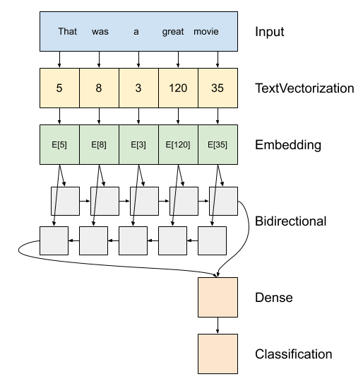
Powyżej znajduje się schemat modelu.
Model ten może być build jako
tf.keras.Sequential.Pierwsza warstwa jest
encoder, który przekształca tekst sekwencji wskaźników znaczników.Po koderze jest warstwa osadzania. Warstwa osadzania przechowuje jeden wektor na słowo. Po wywołaniu konwertuje sekwencje indeksów słów na sekwencje wektorów. Te wektory można trenować. Po przeszkoleniu (na wystarczającej ilości danych) słowa o podobnym znaczeniu mają często podobne wektory.
Ten indeksu wyszukiwania jest znacznie bardziej skuteczny niż równoważne działanie przechodząc jedną gorącą kodowanego przez wektor
tf.keras.layers.Densewarstwy.Rekurencyjna sieć neuronowa (RNN) przetwarza dane wejściowe sekwencji poprzez iterację przez elementy. RNN przekazują dane wyjściowe z jednego kroku czasowego do swoich danych wejściowych w następnym kroku czasowym.
tf.keras.layers.BidirectionalOwijka może być również stosowany z warstwą RNN. Powoduje to propagację danych wejściowych do przodu i do tyłu przez warstwę RNN, a następnie łączy końcowy wynik.Główną zaletą dwukierunkowego RNN jest to, że sygnał z początku wejścia nie musi być przetwarzany w każdym kroku czasowym, aby wpłynąć na wyjście.
Główną wadą dwukierunkowej sieci RNN jest to, że nie można wydajnie przesyłać podpowiedzi, ponieważ słowa są dodawane na końcu.
Po RNN przeszła sekwencję do jednego wektora dwa
layers.Densezrobić końcowego przetwarzania, i przekształcenia z tej reprezentacji wektora do jednego logit jako wyjście klasyfikacji.
Kod do wdrożenia tego znajduje się poniżej:
model = tf.keras.Sequential([
    encoder,
    tf.keras.layers.Embedding(
        input_dim=len(encoder.get_vocabulary()),
        output_dim=64,
        # Use masking to handle the variable sequence lengths
        mask_zero=True),
    tf.keras.layers.Bidirectional(tf.keras.layers.LSTM(64)),
    tf.keras.layers.Dense(64, activation='relu'),
    tf.keras.layers.Dense(1)
])
Należy pamiętać, że zastosowano tutaj model sekwencyjny Keras, ponieważ wszystkie warstwy w modelu mają tylko jedno wejście i produkują jedno wyjście. Jeśli chcesz użyć stanowej warstwy RNN, możesz zbudować swój model za pomocą funkcjonalnego interfejsu API Keras lub podklasy modeli, aby można było pobierać i ponownie wykorzystywać stany warstwy RNN. Proszę sprawdzić Keras RNN przewodnik po więcej szczegółów.
Osadzanie warstwy zastosowania maskowania aby obsługiwać różne od sekwencji długości. Wszystkie warstwy po Embedding wsparcia maskowania:
print([layer.supports_masking for layer in model.layers])
[False, True, True, True, True]
Aby potwierdzić, że działa to zgodnie z oczekiwaniami, dwukrotnie oceń zdanie. Po pierwsze, sam, więc nie ma wyściółki do zamaskowania:
# predict on a sample text without padding.

sample_text = ('The movie was cool. The animation and the graphics '
               'were out of this world. I would recommend this movie.')
predictions = model.predict(np.array([sample_text]))
print(predictions[0])
[-0.00012211]
Teraz oceń to ponownie w partii z dłuższym zdaniem. Wynik powinien być identyczny:
# predict on a sample text with padding

padding = "the " * 2000
predictions = model.predict(np.array([sample_text, padding]))
print(predictions[0])
[-0.00012211]
Skompiluj model Keras, aby skonfigurować proces uczenia:
model.compile(loss=tf.keras.losses.BinaryCrossentropy(from_logits=True),
              optimizer=tf.keras.optimizers.Adam(1e-4),
              metrics=['accuracy'])
Trenuj modelkę
history = model.fit(train_dataset, epochs=10,
                    validation_data=test_dataset,
                    validation_steps=30)
Epoch 1/10
391/391 [==============================] - 39s 84ms/step - loss: 0.6454 - accuracy: 0.5630 - val_loss: 0.4888 - val_accuracy: 0.7568
Epoch 2/10
391/391 [==============================] - 30s 75ms/step - loss: 0.3925 - accuracy: 0.8200 - val_loss: 0.3663 - val_accuracy: 0.8464
Epoch 3/10
391/391 [==============================] - 30s 75ms/step - loss: 0.3319 - accuracy: 0.8525 - val_loss: 0.3402 - val_accuracy: 0.8385
Epoch 4/10
391/391 [==============================] - 30s 75ms/step - loss: 0.3183 - accuracy: 0.8616 - val_loss: 0.3289 - val_accuracy: 0.8438
Epoch 5/10
391/391 [==============================] - 30s 75ms/step - loss: 0.3088 - accuracy: 0.8656 - val_loss: 0.3254 - val_accuracy: 0.8646
Epoch 6/10
391/391 [==============================] - 32s 81ms/step - loss: 0.3043 - accuracy: 0.8686 - val_loss: 0.3242 - val_accuracy: 0.8521
Epoch 7/10
391/391 [==============================] - 30s 76ms/step - loss: 0.3019 - accuracy: 0.8696 - val_loss: 0.3315 - val_accuracy: 0.8609
Epoch 8/10
391/391 [==============================] - 32s 76ms/step - loss: 0.3007 - accuracy: 0.8688 - val_loss: 0.3245 - val_accuracy: 0.8609
Epoch 9/10
391/391 [==============================] - 31s 77ms/step - loss: 0.2981 - accuracy: 0.8707 - val_loss: 0.3294 - val_accuracy: 0.8599
Epoch 10/10
391/391 [==============================] - 31s 78ms/step - loss: 0.2969 - accuracy: 0.8742 - val_loss: 0.3218 - val_accuracy: 0.8547
test_loss, test_acc = model.evaluate(test_dataset)

print('Test Loss:', test_loss)
print('Test Accuracy:', test_acc)
391/391 [==============================] - 15s 38ms/step - loss: 0.3185 - accuracy: 0.8582
Test Loss: 0.3184521794319153
Test Accuracy: 0.8581600189208984
plt.figure(figsize=(16, 8))
plt.subplot(1, 2, 1)
plot_graphs(history, 'accuracy')
plt.ylim(None, 1)
plt.subplot(1, 2, 2)
plot_graphs(history, 'loss')
plt.ylim(0, None)
(0.0, 0.6627909764647484)

Uruchom przewidywanie nowego zdania:
Jeśli prognoza jest >= 0.0, jest dodatnia, w przeciwnym razie jest ujemna.
sample_text = ('The movie was cool. The animation and the graphics '
               'were out of this world. I would recommend this movie.')
predictions = model.predict(np.array([sample_text]))
Ułóż dwie lub więcej warstw LSTM
Keras nawracające warstwy mają dwa dostępne tryby, które są kontrolowane przez return_sequences argument konstruktora:
Jeśli
Falsezwraca tylko ostatni wyjście dla każdej sekwencji wejściowej (2D tensor kształtu (batch_size, output_features)). Jest to ustawienie domyślne używane w poprzednim modelu.Jeśli
Truepełne sekwencje kolejnych wyjściowych dla każdego kroku to jest zwracana (tensora 3D kształtu(batch_size, timesteps, output_features)).
Oto co przepływ informacji wygląda jak z return_sequences=True :
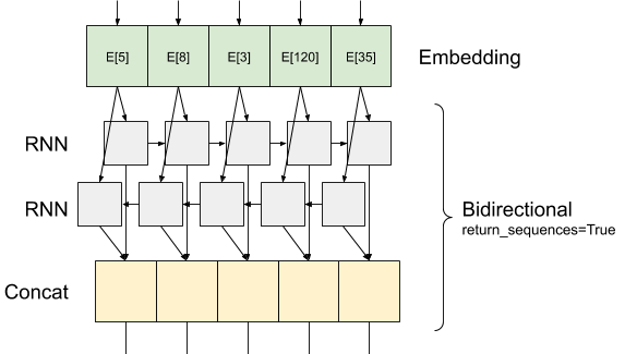
Interesującą rzeczą przy użyciu RNN z return_sequences=True to, że wyjście nadal ma 3-osiowa, jak wejścia, więc to może być przekazane do innej warstwy RNN, jak poniżej:
model = tf.keras.Sequential([
    encoder,
    tf.keras.layers.Embedding(len(encoder.get_vocabulary()), 64, mask_zero=True),
    tf.keras.layers.Bidirectional(tf.keras.layers.LSTM(64,  return_sequences=True)),
    tf.keras.layers.Bidirectional(tf.keras.layers.LSTM(32)),
    tf.keras.layers.Dense(64, activation='relu'),
    tf.keras.layers.Dropout(0.5),
    tf.keras.layers.Dense(1)
])
model.compile(loss=tf.keras.losses.BinaryCrossentropy(from_logits=True),
              optimizer=tf.keras.optimizers.Adam(1e-4),
              metrics=['accuracy'])
history = model.fit(train_dataset, epochs=10,
                    validation_data=test_dataset,
                    validation_steps=30)
Epoch 1/10
391/391 [==============================] - 71s 149ms/step - loss: 0.6502 - accuracy: 0.5625 - val_loss: 0.4923 - val_accuracy: 0.7573
Epoch 2/10
391/391 [==============================] - 55s 138ms/step - loss: 0.4067 - accuracy: 0.8198 - val_loss: 0.3727 - val_accuracy: 0.8271
Epoch 3/10
391/391 [==============================] - 54s 136ms/step - loss: 0.3417 - accuracy: 0.8543 - val_loss: 0.3343 - val_accuracy: 0.8510
Epoch 4/10
391/391 [==============================] - 53s 134ms/step - loss: 0.3242 - accuracy: 0.8607 - val_loss: 0.3268 - val_accuracy: 0.8568
Epoch 5/10
391/391 [==============================] - 53s 135ms/step - loss: 0.3174 - accuracy: 0.8652 - val_loss: 0.3213 - val_accuracy: 0.8516
Epoch 6/10
391/391 [==============================] - 52s 132ms/step - loss: 0.3098 - accuracy: 0.8671 - val_loss: 0.3294 - val_accuracy: 0.8547
Epoch 7/10
391/391 [==============================] - 53s 134ms/step - loss: 0.3063 - accuracy: 0.8697 - val_loss: 0.3158 - val_accuracy: 0.8594
Epoch 8/10
391/391 [==============================] - 52s 132ms/step - loss: 0.3043 - accuracy: 0.8692 - val_loss: 0.3184 - val_accuracy: 0.8521
Epoch 9/10
391/391 [==============================] - 53s 133ms/step - loss: 0.3016 - accuracy: 0.8704 - val_loss: 0.3208 - val_accuracy: 0.8609
Epoch 10/10
391/391 [==============================] - 54s 136ms/step - loss: 0.2975 - accuracy: 0.8740 - val_loss: 0.3301 - val_accuracy: 0.8651
test_loss, test_acc = model.evaluate(test_dataset)

print('Test Loss:', test_loss)
print('Test Accuracy:', test_acc)
391/391 [==============================] - 26s 65ms/step - loss: 0.3293 - accuracy: 0.8646
Test Loss: 0.329334557056427
Test Accuracy: 0.8646399974822998
# predict on a sample text without padding.

sample_text = ('The movie was not good. The animation and the graphics '
               'were terrible. I would not recommend this movie.')
predictions = model.predict(np.array([sample_text]))
print(predictions)
[[-1.6796288]]
plt.figure(figsize=(16, 6))
plt.subplot(1, 2, 1)
plot_graphs(history, 'accuracy')
plt.subplot(1, 2, 2)
plot_graphs(history, 'loss')

Sprawdź inne istniejących warstw, takich jak nawracające warstw GRU .
Jeśli interestied budowania niestandardowych RNNs, zobacz Keras RNN Guide .