उन्नत स्वचालित भेदभाव

TensorFlow.org पर देखें

Google Colab में चलाएं

GitHub पर स्रोत देखें

नोटबुक डाउनलोड करें

ग्रेडिएंट का परिचय और स्वचालित विभेदन मार्गदर्शिका में TensorFlow में ग्रेडिएंट की गणना करने के लिए आवश्यक सभी चीजें शामिल हैं। यह मार्गदर्शिका tf.GradientTape API की गहरी, कम सामान्य विशेषताओं पर केंद्रित है।

सेट अप

import tensorflow as tf

import matplotlib as mpl
import matplotlib.pyplot as plt

mpl.rcParams['figure.figsize'] = (8, 6)

ग्रेडिएंट रिकॉर्डिंग को नियंत्रित करना

स्वचालित विभेदन मार्गदर्शिका में आपने देखा कि ग्रेडिएंट गणना का निर्माण करते समय टेप द्वारा कौन से चर और टेंसर देखे जाते हैं, इसे कैसे नियंत्रित किया जाए।

टेप में रिकॉर्डिंग में हेरफेर करने के तरीके भी हैं।

रिकॉर्डिंग बंद करें

यदि आप ग्रेडिएंट की रिकॉर्डिंग बंद करना चाहते हैं, तो आप रिकॉर्डिंग को अस्थायी रूप से निलंबित करने के लिए tf.GradientTape.stop_recording का उपयोग कर सकते हैं।

यदि आप अपने मॉडल के बीच में एक जटिल ऑपरेशन को अलग नहीं करना चाहते हैं तो यह ओवरहेड को कम करने के लिए उपयोगी हो सकता है। इसमें मीट्रिक या मध्यवर्ती परिणाम की गणना करना शामिल हो सकता है:

x = tf.Variable(2.0)
y = tf.Variable(3.0)

with tf.GradientTape() as t:
  x_sq = x * x
  with t.stop_recording():
    y_sq = y * y
  z = x_sq + y_sq

grad = t.gradient(z, {'x': x, 'y': y})

print('dz/dx:', grad['x'])  # 2*x => 4
print('dz/dy:', grad['y'])

dz/dx: tf.Tensor(4.0, shape=(), dtype=float32)
dz/dy: None

खरोंच से रिकॉर्डिंग रीसेट/शुरू करें

यदि आप पूरी तरह से शुरू करना चाहते हैं, तो tf.GradientTape.reset का उपयोग करें। बस ग्रेडिएंट टेप ब्लॉक से बाहर निकलना और फिर से शुरू करना आमतौर पर पढ़ने में आसान होता है, लेकिन जब टेप ब्लॉक से बाहर निकलना मुश्किल या असंभव हो तो आप reset विधि का उपयोग कर सकते हैं।

x = tf.Variable(2.0)
y = tf.Variable(3.0)
reset = True

with tf.GradientTape() as t:
  y_sq = y * y
  if reset:
    # Throw out all the tape recorded so far.
    t.reset()
  z = x * x + y_sq

grad = t.gradient(z, {'x': x, 'y': y})

print('dz/dx:', grad['x'])  # 2*x => 4
print('dz/dy:', grad['y'])

dz/dx: tf.Tensor(4.0, shape=(), dtype=float32)
dz/dy: None

परिशुद्धता के साथ ढाल प्रवाह रोकें

उपरोक्त वैश्विक टेप नियंत्रणों के विपरीत, tf.stop_gradient फ़ंक्शन अधिक सटीक है। इसका उपयोग ग्रेडियेंट को किसी विशेष पथ के साथ बहने से रोकने के लिए किया जा सकता है, बिना टेप तक पहुंच की आवश्यकता के:

x = tf.Variable(2.0)
y = tf.Variable(3.0)

with tf.GradientTape() as t:
  y_sq = y**2
  z = x**2 + tf.stop_gradient(y_sq)

grad = t.gradient(z, {'x': x, 'y': y})

print('dz/dx:', grad['x'])  # 2*x => 4
print('dz/dy:', grad['y'])

dz/dx: tf.Tensor(4.0, shape=(), dtype=float32)
dz/dy: None

कस्टम ग्रेडिएंट

कुछ मामलों में, आप यह नियंत्रित करना चाह सकते हैं कि डिफ़ॉल्ट का उपयोग करने के बजाय ग्रेडिएंट की गणना कैसे की जाती है। इन स्थितियों में शामिल हैं:

1. आपके द्वारा लिखे जा रहे नए ऑप के लिए कोई परिभाषित ग्रेडिएंट नहीं है।
2. डिफ़ॉल्ट गणना संख्यात्मक रूप से अस्थिर है।
3. आप फॉरवर्ड पास से एक महंगी गणना को कैश करना चाहते हैं।
4. आप ग्रेडिएंट को संशोधित किए बिना किसी मान को संशोधित करना चाहते हैं (उदाहरण के लिए, tf.clip_by_value या tf.math.round का उपयोग करके)।

पहले मामले के लिए, एक नया ऑप लिखने के लिए आप अपना खुद का सेट करने के लिए tf.RegisterGradient का उपयोग कर सकते हैं (विवरण के लिए एपीआई डॉक्स देखें)। (ध्यान दें कि ग्रेडिएंट रजिस्ट्री वैश्विक है, इसलिए इसे सावधानी के साथ बदलें।)

बाद के तीन मामलों के लिए, आप tf.custom_gradient का उपयोग कर सकते हैं।

यहां एक उदाहरण दिया गया है जो tf.clip_by_norm को इंटरमीडिएट ग्रेडिएंट पर लागू करता है:

# Establish an identity operation, but clip during the gradient pass.
@tf.custom_gradient
def clip_gradients(y):
  def backward(dy):
    return tf.clip_by_norm(dy, 0.5)
  return y, backward

v = tf.Variable(2.0)
with tf.GradientTape() as t:
  output = clip_gradients(v * v)
print(t.gradient(output, v))  # calls "backward", which clips 4 to 2

tf.Tensor(2.0, shape=(), dtype=float32)

अधिक विवरण के लिए tf.custom_gradient डेकोरेटर API दस्तावेज़ देखें।

सहेजे गए मॉडल में कस्टम ग्रेडिएंट

tf.saved_model.SaveOptions(experimental_custom_gradients=True) विकल्प का उपयोग करके कस्टम ग्रेडिएंट को SavedModel में सहेजा जा सकता है।

सहेजे गए मॉडल में सहेजे जाने के लिए, ग्रेडिएंट फ़ंक्शन का पता लगाने योग्य होना चाहिए (अधिक जानने के लिए, tf.function मार्गदर्शिका के साथ बेहतर प्रदर्शन देखें )।

class MyModule(tf.Module):

  @tf.function(input_signature=[tf.TensorSpec(None)])
  def call_custom_grad(self, x):
    return clip_gradients(x)

model = MyModule()

tf.saved_model.save(
    model,
    'saved_model',
    options=tf.saved_model.SaveOptions(experimental_custom_gradients=True))

# The loaded gradients will be the same as the above example.
v = tf.Variable(2.0)
loaded = tf.saved_model.load('saved_model')
with tf.GradientTape() as t:
  output = loaded.call_custom_grad(v * v)
print(t.gradient(output, v))

INFO:tensorflow:Assets written to: saved_model/assets
tf.Tensor(2.0, shape=(), dtype=float32)

उपरोक्त उदाहरण के बारे में एक नोट: यदि आप उपरोक्त कोड को tf.saved_model.SaveOptions(experimental_custom_gradients=False) से बदलने का प्रयास करते हैं, तो ग्रेडिएंट लोड होने पर भी वही परिणाम देगा। कारण यह है कि ग्रेडिएंट रजिस्ट्री में अभी भी call_custom_op फ़ंक्शन में उपयोग किया जाने वाला कस्टम ग्रेडिएंट है। हालांकि, यदि आप कस्टम ग्रेडिएंट के बिना सहेजने के बाद रनटाइम को पुनरारंभ करते हैं, तो tf.GradientTape के तहत लोड किए गए मॉडल को चलाने से त्रुटि होगी: लुकअप एरर: LookupError: No gradient defined for operation 'IdentityN' (op type: IdentityN) ।

एकाधिक टेप

एकाधिक टेप निर्बाध रूप से इंटरैक्ट करते हैं।

उदाहरण के लिए, यहां प्रत्येक टेप टेंसर का एक अलग सेट देखता है:

x0 = tf.constant(0.0)
x1 = tf.constant(0.0)

with tf.GradientTape() as tape0, tf.GradientTape() as tape1:
  tape0.watch(x0)
  tape1.watch(x1)

  y0 = tf.math.sin(x0)
  y1 = tf.nn.sigmoid(x1)

  y = y0 + y1

  ys = tf.reduce_sum(y)

tape0.gradient(ys, x0).numpy()   # cos(x) => 1.0

1.0

tape1.gradient(ys, x1).numpy()   # sigmoid(x1)*(1-sigmoid(x1)) => 0.25

0.25

उच्च-क्रम के ग्रेडिएंट

tf.GradientTape संदर्भ प्रबंधक के अंदर के संचालन स्वचालित भेदभाव के लिए रिकॉर्ड किए जाते हैं। यदि उस संदर्भ में ग्रेडिएंट की गणना की जाती है, तो ग्रेडिएंट गणना भी दर्ज की जाती है। नतीजतन, ठीक वही एपीआई उच्च-क्रम वाले ग्रेडिएंट के लिए भी काम करता है।

उदाहरण के लिए:

x = tf.Variable(1.0)  # Create a Tensorflow variable initialized to 1.0

with tf.GradientTape() as t2:
  with tf.GradientTape() as t1:
    y = x * x * x

  # Compute the gradient inside the outer `t2` context manager
  # which means the gradient computation is differentiable as well.
  dy_dx = t1.gradient(y, x)
d2y_dx2 = t2.gradient(dy_dx, x)

print('dy_dx:', dy_dx.numpy())  # 3 * x**2 => 3.0
print('d2y_dx2:', d2y_dx2.numpy())  # 6 * x => 6.0

dy_dx: 3.0
d2y_dx2: 6.0

जबकि यह आपको स्केलर फ़ंक्शन का दूसरा व्युत्पन्न देता है, यह पैटर्न हेसियन मैट्रिक्स का उत्पादन करने के लिए सामान्यीकृत नहीं करता है, क्योंकि tf.GradientTape.gradient केवल एक स्केलर के ग्रेडिएंट की गणना करता है। हेसियन मैट्रिक्स का निर्माण करने के लिए, जैकोबियन सेक्शन के तहत हेसियन उदाहरण पर जाएं।

" tf.GradientTape.gradient के लिए नेस्टेड कॉल" एक अच्छा पैटर्न है जब आप एक ग्रेडिएंट से स्केलर की गणना कर रहे हैं, और फिर परिणामी स्केलर दूसरी ग्रेडिएंट गणना के लिए एक स्रोत के रूप में कार्य करता है, जैसा कि निम्नलिखित उदाहरण में है।

उदाहरण: इनपुट ग्रेडिएंट नियमितीकरण

कई मॉडल "प्रतिकूल उदाहरण" के लिए अतिसंवेदनशील होते हैं। तकनीकों का यह संग्रह मॉडल के आउटपुट को भ्रमित करने के लिए मॉडल के इनपुट को संशोधित करता है। सबसे सरल कार्यान्वयन- जैसे कि फास्ट ग्रेडिएंट साइन्ड मेथड अटैक का उपयोग करने वाला एडवरसैरियल उदाहरण - इनपुट के संबंध में आउटपुट के ग्रेडिएंट के साथ एक ही कदम उठाता है; "इनपुट ग्रेडिएंट"।

प्रतिकूल उदाहरणों के लिए मजबूती बढ़ाने की एक तकनीक इनपुट ग्रेडिएंट रेगुलराइजेशन (फिनले एंड ओबरमैन, 2019) है, जो इनपुट ग्रेडिएंट के परिमाण को कम करने का प्रयास करती है। यदि इनपुट ग्रेडिएंट छोटा है, तो आउटपुट में परिवर्तन भी छोटा होना चाहिए।

नीचे इनपुट ग्रेडिएंट नियमितीकरण का एक सरल कार्यान्वयन है। कार्यान्वयन है:

1. एक आंतरिक टेप का उपयोग करके इनपुट के संबंध में आउटपुट के ग्रेडिएंट की गणना करें।
2. उस इनपुट ग्रेडिएंट के परिमाण की गणना करें।
3. मॉडल के संबंध में उस परिमाण के ढाल की गणना करें।

x = tf.random.normal([7, 5])

layer = tf.keras.layers.Dense(10, activation=tf.nn.relu)

with tf.GradientTape() as t2:
  # The inner tape only takes the gradient with respect to the input,
  # not the variables.
  with tf.GradientTape(watch_accessed_variables=False) as t1:
    t1.watch(x)
    y = layer(x)
    out = tf.reduce_sum(layer(x)**2)
  # 1. Calculate the input gradient.
  g1 = t1.gradient(out, x)
  # 2. Calculate the magnitude of the input gradient.
  g1_mag = tf.norm(g1)

# 3. Calculate the gradient of the magnitude with respect to the model.
dg1_mag = t2.gradient(g1_mag, layer.trainable_variables)

[var.shape for var in dg1_mag]

[TensorShape([5, 10]), TensorShape([10])]

जैकोबियन

पिछले सभी उदाहरणों ने कुछ स्रोत टेंसर (ओं) के संबंध में एक स्केलर लक्ष्य के ग्रेडियेंट को लिया।

जैकोबियन मैट्रिक्स एक वेक्टर मान फ़ंक्शन के ग्रेडिएंट का प्रतिनिधित्व करता है। प्रत्येक पंक्ति में वेक्टर के तत्वों में से एक का ग्रेडिएंट होता है।

tf.GradientTape.jacobian विधि आपको एक जैकोबियन मैट्रिक्स की कुशलता से गणना करने की अनुमति देती है।

ध्यान दें कि:

• gradient की तरह: sources तर्क एक टेंसर या टेंसर का एक कंटेनर हो सकता है।
• gradient के विपरीत: target टेंसर एक सिंगल टेंसर होना चाहिए।

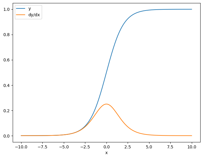
अदिश स्रोत

पहले उदाहरण के रूप में, यहां एक स्केलर-स्रोत के संबंध में वेक्टर-लक्ष्य का जैकोबियन है।

x = tf.linspace(-10.0, 10.0, 200+1)
delta = tf.Variable(0.0)

with tf.GradientTape() as tape:
  y = tf.nn.sigmoid(x+delta)

dy_dx = tape.jacobian(y, delta)

जब आप जैकोबियन को स्केलर के संबंध में लेते हैं तो परिणाम में लक्ष्य का आकार होता है, और स्रोत के संबंध में प्रत्येक तत्व की ढाल देता है:

print(y.shape)
print(dy_dx.shape)

(201,)
(201,)

प्लेसहोल्डर26 l10n-प्लेसहोल्डर

plt.plot(x.numpy(), y, label='y')
plt.plot(x.numpy(), dy_dx, label='dy/dx')
plt.legend()
_ = plt.xlabel('x')

टेंसर स्रोत

चाहे इनपुट स्केलर हो या टेंसर, tf.GradientTape.jacobian लक्ष्य के प्रत्येक तत्व के संबंध में स्रोत के प्रत्येक तत्व के ग्रेडिएंट की कुशलता से गणना करता है।

उदाहरण के लिए, इस परत के आउटपुट का आकार (10, 7) :

x = tf.random.normal([7, 5])
layer = tf.keras.layers.Dense(10, activation=tf.nn.relu)

with tf.GradientTape(persistent=True) as tape:
  y = layer(x)

y.shape

TensorShape([7, 10])

और परत की गुठली का आकार होता है (5, 10) :

layer.kernel.shape

TensorShape([5, 10])

कर्नेल के संबंध में आउटपुट के जैकोबियन का आकार वे दो आकार हैं जो एक साथ जुड़े हुए हैं:

j = tape.jacobian(y, layer.kernel)
j.shape

TensorShape([7, 10, 5, 10])

प्लेसहोल्डर33

यदि आप लक्ष्य के आयामों पर योग करते हैं, तो आपके पास उस योग के ग्रेडिएंट के साथ छोड़ दिया जाता है जिसकी गणना tf.GradientTape.gradient द्वारा की जाती है:

g = tape.gradient(y, layer.kernel)
print('g.shape:', g.shape)

j_sum = tf.reduce_sum(j, axis=[0, 1])
delta = tf.reduce_max(abs(g - j_sum)).numpy()
assert delta < 1e-3
print('delta:', delta)

34 एल10एन-प्लेसहोल्डर

g.shape: (5, 10)
delta: 2.3841858e-07

उदाहरण: हेसियन

जबकि tf.GradientTape एक हेसियन मैट्रिक्स के निर्माण के लिए एक स्पष्ट विधि नहीं देता है, tf.GradientTape.jacobian पद्धति का उपयोग करके इसे बनाना संभव है।

x = tf.random.normal([7, 5])
layer1 = tf.keras.layers.Dense(8, activation=tf.nn.relu)
layer2 = tf.keras.layers.Dense(6, activation=tf.nn.relu)

with tf.GradientTape() as t2:
  with tf.GradientTape() as t1:
    x = layer1(x)
    x = layer2(x)
    loss = tf.reduce_mean(x**2)

  g = t1.gradient(loss, layer1.kernel)

h = t2.jacobian(g, layer1.kernel)

print(f'layer.kernel.shape: {layer1.kernel.shape}')
print(f'h.shape: {h.shape}')

layer.kernel.shape: (5, 8)
h.shape: (5, 8, 5, 8)

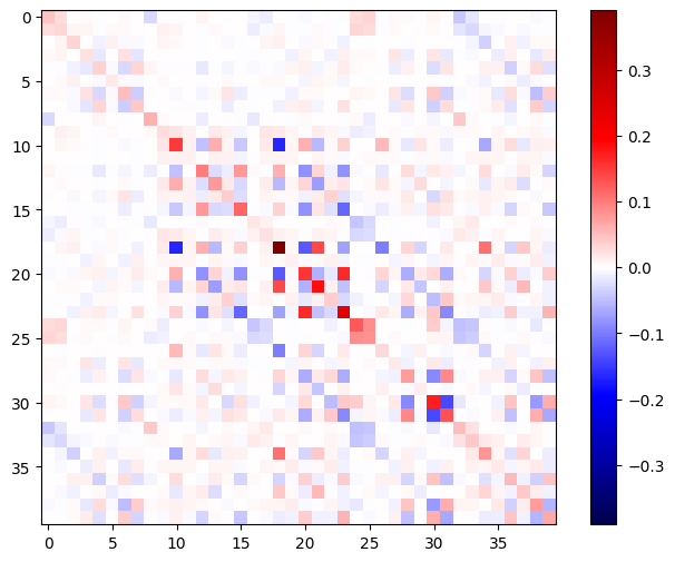
न्यूटन के विधि चरण के लिए इस हेसियन का उपयोग करने के लिए, आप पहले इसकी कुल्हाड़ियों को एक मैट्रिक्स में समतल करेंगे, और ग्रेडिएंट को एक वेक्टर में समतल करेंगे:

n_params = tf.reduce_prod(layer1.kernel.shape)

g_vec = tf.reshape(g, [n_params, 1])
h_mat = tf.reshape(h, [n_params, n_params])

हेसियन मैट्रिक्स सममित होना चाहिए:

def imshow_zero_center(image, **kwargs):
  lim = tf.reduce_max(abs(image))
  plt.imshow(image, vmin=-lim, vmax=lim, cmap='seismic', **kwargs)
  plt.colorbar()

imshow_zero_center(h_mat)

न्यूटन की विधि अद्यतन चरण नीचे दिखाया गया है:

eps = 1e-3
eye_eps = tf.eye(h_mat.shape[0])*eps

# X(k+1) = X(k) - (∇²f(X(k)))^-1 @ ∇f(X(k))
# h_mat = ∇²f(X(k))
# g_vec = ∇f(X(k))
update = tf.linalg.solve(h_mat + eye_eps, g_vec)

# Reshape the update and apply it to the variable.
_ = layer1.kernel.assign_sub(tf.reshape(update, layer1.kernel.shape))

हालांकि यह एक tf.Variable के लिए अपेक्षाकृत सरल है, इसे गैर-तुच्छ मॉडल पर लागू करने के लिए कई चरों में एक पूर्ण हेसियन का उत्पादन करने के लिए सावधानीपूर्वक संयोजन और स्लाइसिंग की आवश्यकता होगी।

बैच जैकोबियन

कुछ मामलों में, आप स्रोतों के ढेर के संबंध में लक्ष्य के प्रत्येक स्टैक का जैकोबियन लेना चाहते हैं, जहां प्रत्येक लक्ष्य-स्रोत जोड़ी के लिए जैकोबियन स्वतंत्र होते हैं।

उदाहरण के लिए, यहां इनपुट x को आकार दिया गया है (batch, ins) और आउटपुट y को आकार दिया गया है (batch, outs) :

x = tf.random.normal([7, 5])

layer1 = tf.keras.layers.Dense(8, activation=tf.nn.elu)
layer2 = tf.keras.layers.Dense(6, activation=tf.nn.elu)

with tf.GradientTape(persistent=True, watch_accessed_variables=False) as tape:
  tape.watch(x)
  y = layer1(x)
  y = layer2(y)

y.shape

TensorShape([7, 6])

x के संबंध में y के पूर्ण जैकोबियन का आकार (batch, ins, batch, outs) , भले ही आप केवल (batch, ins, outs) चाहते हों:

j = tape.jacobian(y, x)
j.shape

TensorShape([7, 6, 7, 5])

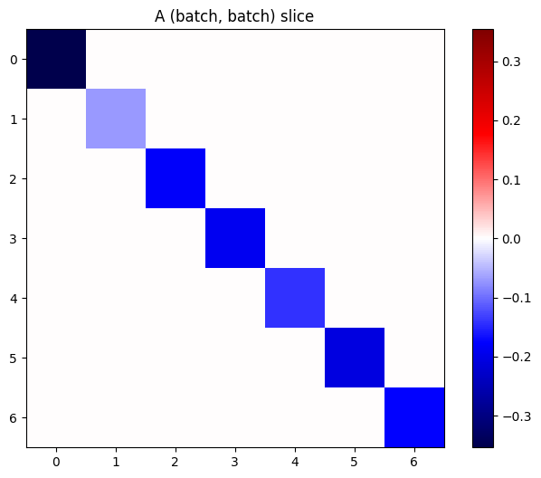
यदि स्टैक में प्रत्येक आइटम के ग्रेडिएंट स्वतंत्र हैं, तो इस टेंसर का प्रत्येक (batch, batch) टुकड़ा एक विकर्ण मैट्रिक्स है:

imshow_zero_center(j[:, 0, :, 0])
_ = plt.title('A (batch, batch) slice')

def plot_as_patches(j):
  # Reorder axes so the diagonals will each form a contiguous patch.
  j = tf.transpose(j, [1, 0, 3, 2])
  # Pad in between each patch.
  lim = tf.reduce_max(abs(j))
  j = tf.pad(j, [[0, 0], [1, 1], [0, 0], [1, 1]],
             constant_values=-lim)
  # Reshape to form a single image.
  s = j.shape
  j = tf.reshape(j, [s[0]*s[1], s[2]*s[3]])
  imshow_zero_center(j, extent=[-0.5, s[2]-0.5, s[0]-0.5, -0.5])

plot_as_patches(j)
_ = plt.title('All (batch, batch) slices are diagonal')

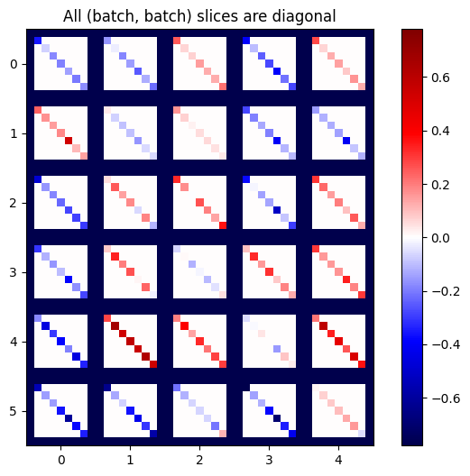
वांछित परिणाम प्राप्त करने के लिए, आप डुप्लिकेट batch आयाम पर योग कर सकते हैं, या फिर tf.einsum का उपयोग करके विकर्णों का चयन कर सकते हैं:

j_sum = tf.reduce_sum(j, axis=2)
print(j_sum.shape)
j_select = tf.einsum('bxby->bxy', j)
print(j_select.shape)

(7, 6, 5)
(7, 6, 5)

पहली जगह में अतिरिक्त आयाम के बिना गणना करना अधिक कुशल होगा। tf.GradientTape.batch_jacobian विधि ठीक यही करती है:

jb = tape.batch_jacobian(y, x)
jb.shape

WARNING:tensorflow:5 out of the last 5 calls to <function pfor.<locals>.f at 0x7f7d601250e0> triggered tf.function retracing. Tracing is expensive and the excessive number of tracings could be due to (1) creating @tf.function repeatedly in a loop, (2) passing tensors with different shapes, (3) passing Python objects instead of tensors. For (1), please define your @tf.function outside of the loop. For (2), @tf.function has experimental_relax_shapes=True option that relaxes argument shapes that can avoid unnecessary retracing. For (3), please refer to https://www.tensorflow.org/guide/function#controlling_retracing and https://www.tensorflow.org/api_docs/python/tf/function for  more details.
TensorShape([7, 6, 5])

error = tf.reduce_max(abs(jb - j_sum))
assert error < 1e-3
print(error.numpy())

0.0

x = tf.random.normal([7, 5])

layer1 = tf.keras.layers.Dense(8, activation=tf.nn.elu)
bn = tf.keras.layers.BatchNormalization()
layer2 = tf.keras.layers.Dense(6, activation=tf.nn.elu)

with tf.GradientTape(persistent=True, watch_accessed_variables=False) as tape:
  tape.watch(x)
  y = layer1(x)
  y = bn(y, training=True)
  y = layer2(y)

j = tape.jacobian(y, x)
print(f'j.shape: {j.shape}')

WARNING:tensorflow:6 out of the last 6 calls to <function pfor.<locals>.f at 0x7f7cf062fa70> triggered tf.function retracing. Tracing is expensive and the excessive number of tracings could be due to (1) creating @tf.function repeatedly in a loop, (2) passing tensors with different shapes, (3) passing Python objects instead of tensors. For (1), please define your @tf.function outside of the loop. For (2), @tf.function has experimental_relax_shapes=True option that relaxes argument shapes that can avoid unnecessary retracing. For (3), please refer to https://www.tensorflow.org/guide/function#controlling_retracing and https://www.tensorflow.org/api_docs/python/tf/function for  more details.
j.shape: (7, 6, 7, 5)

plot_as_patches(j)

_ = plt.title('These slices are not diagonal')
_ = plt.xlabel("Don't use `batch_jacobian`")

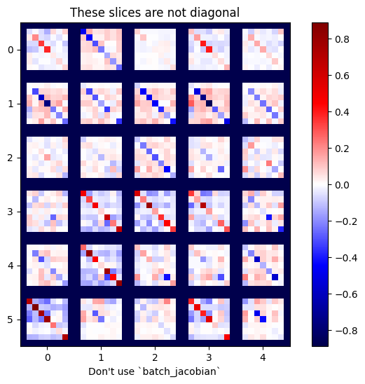
इस मामले में, batch_jacobian अभी भी चलता है और अपेक्षित आकार के साथ कुछ देता है, लेकिन इसकी सामग्री का एक अस्पष्ट अर्थ है:

jb = tape.batch_jacobian(y, x)
print(f'jb.shape: {jb.shape}')

jb.shape: (7, 6, 5)