
|
|
|
 View source on GitHub View source on GitHub
|
|
This guide provides a quick overview of TensorFlow basics. Each section of this doc is an overview of a larger topic—you can find links to full guides at the end of each section.
TensorFlow is an end-to-end platform for machine learning. It supports the following:
- Multidimensional-array based numeric computation (similar to NumPy.)
- GPU and distributed processing
- Automatic differentiation
- Model construction, training, and export
- And more
Tensors
TensorFlow operates on multidimensional arrays or tensors represented as tf.Tensor objects. Here is a two-dimensional tensor:
import tensorflow as tf

x = tf.constant([[1., 2., 3.],
                 [4., 5., 6.]])

print(x)
print(x.shape)
print(x.dtype)
2024-10-03 01:24:28.897515: E external/local_xla/xla/stream_executor/cuda/cuda_fft.cc:485] Unable to register cuFFT factory: Attempting to register factory for plugin cuFFT when one has already been registered
2024-10-03 01:24:28.918497: E external/local_xla/xla/stream_executor/cuda/cuda_dnn.cc:8454] Unable to register cuDNN factory: Attempting to register factory for plugin cuDNN when one has already been registered
2024-10-03 01:24:28.924727: E external/local_xla/xla/stream_executor/cuda/cuda_blas.cc:1452] Unable to register cuBLAS factory: Attempting to register factory for plugin cuBLAS when one has already been registered
WARNING: All log messages before absl::InitializeLog() is called are written to STDERR
I0000 00:00:1727918671.501067   10533 cuda_executor.cc:1015] successful NUMA node read from SysFS had negative value (-1), but there must be at least one NUMA node, so returning NUMA node zero. See more at https://github.com/torvalds/linux/blob/v6.0/Documentation/ABI/testing/sysfs-bus-pci#L344-L355
I0000 00:00:1727918671.504962   10533 cuda_executor.cc:1015] successful NUMA node read from SysFS had negative value (-1), but there must be at least one NUMA node, so returning NUMA node zero. See more at https://github.com/torvalds/linux/blob/v6.0/Documentation/ABI/testing/sysfs-bus-pci#L344-L355
I0000 00:00:1727918671.508951   10533 cuda_executor.cc:1015] successful NUMA node read from SysFS had negative value (-1), but there must be at least one NUMA node, so returning NUMA node zero. See more at https://github.com/torvalds/linux/blob/v6.0/Documentation/ABI/testing/sysfs-bus-pci#L344-L355
I0000 00:00:1727918671.512662   10533 cuda_executor.cc:1015] successful NUMA node read from SysFS had negative value (-1), but there must be at least one NUMA node, so returning NUMA node zero. See more at https://github.com/torvalds/linux/blob/v6.0/Documentation/ABI/testing/sysfs-bus-pci#L344-L355
I0000 00:00:1727918671.523975   10533 cuda_executor.cc:1015] successful NUMA node read from SysFS ha
tf.Tensor(
[[1. 2. 3.]
 [4. 5. 6.]], shape=(2, 3), dtype=float32)
(2, 3)
<dtype: 'float32'>
d negative value (-1), but there must be at least one NUMA node, so returning NUMA node zero. See more at https://github.com/torvalds/linux/blob/v6.0/Documentation/ABI/testing/sysfs-bus-pci#L344-L355
I0000 00:00:1727918671.527575   10533 cuda_executor.cc:1015] successful NUMA node read from SysFS had negative value (-1), but there must be at least one NUMA node, so returning NUMA node zero. See more at https://github.com/torvalds/linux/blob/v6.0/Documentation/ABI/testing/sysfs-bus-pci#L344-L355
I0000 00:00:1727918671.531095   10533 cuda_executor.cc:1015] successful NUMA node read from SysFS had negative value (-1), but there must be at least one NUMA node, so returning NUMA node zero. See more at https://github.com/torvalds/linux/blob/v6.0/Documentation/ABI/testing/sysfs-bus-pci#L344-L355
I0000 00:00:1727918671.534452   10533 cuda_executor.cc:1015] successful NUMA node read from SysFS had negative value (-1), but there must be at least one NUMA node, so returning NUMA node zero. See more at https://github.com/torvalds/linux/blob/v6.0/Documentation/ABI/testing/sysfs-bus-pci#L344-L355
I0000 00:00:1727918671.537818   10533 cuda_executor.cc:1015] successful NUMA node read from SysFS had negative value (-1), but there must be at least one NUMA node, so returning NUMA node zero. See more at https://github.com/torvalds/linux/blob/v6.0/Documentation/ABI/testing/sysfs-bus-pci#L344-L355
I0000 00:00:1727918671.541314   10533 cuda_executor.cc:1015] successful NUMA node read from SysFS had negative value (-1), but there must be at least one NUMA node, so returning NUMA node zero. See more at https://github.com/torvalds/linux/blob/v6.0/Documentation/ABI/testing/sysfs-bus-pci#L344-L355
I0000 00:00:1727918671.544748   10533 cuda_executor.cc:1015] successful NUMA node read from SysFS had negative value (-1), but there must be at least one NUMA node, so returning NUMA node zero. See more at https://github.com/torvalds/linux/blob/v6.0/Documentation/ABI/testing/sysfs-bus-pci#L344-L355
I0000 00:00:1727918671.548158   10533 cuda_executor.cc:1015] successful NUMA node read from SysFS had negative value (-1), but there must be at least one NUMA node, so returning NUMA node zero. See more at https://github.com/torvalds/linux/blob/v6.0/Documentation/ABI/testing/sysfs-bus-pci#L344-L355
I0000 00:00:1727918672.811574   10533 cuda_executor.cc:1015] successful NUMA node read from SysFS had negative value (-1), but there must be at least one NUMA node, so returning NUMA node zero. See more at https://github.com/torvalds/linux/blob/v6.0/Documentation/ABI/testing/sysfs-bus-pci#L344-L355
I0000 00:00:1727918672.813683   10533 cuda_executor.cc:1015] successful NUMA node read from SysFS had negative value (-1), but there must be at least one NUMA node, so returning NUMA node zero. See more at https://github.com/torvalds/linux/blob/v6.0/Documentation/ABI/testing/sysfs-bus-pci#L344-L355
I0000 00:00:1727918672.815800   10533 cuda_executor.cc:1015] successful NUMA node read from SysFS had negative value (-1), but there must be at least one NUMA node, so returning NUMA node zero. See more at https://github.com/torvalds/linux/blob/v6.0/Documentation/ABI/testing/sysfs-bus-pci#L344-L355
I0000 00:00:1727918672.817784   10533 cuda_executor.cc:1015] successful NUMA node read from SysFS had negative value (-1), but there must be at least one NUMA node, so returning NUMA node zero. See more at https://github.com/torvalds/linux/blob/v6.0/Documentation/ABI/testing/sysfs-bus-pci#L344-L355
I0000 00:00:1727918672.819747   10533 cuda_executor.cc:1015] successful NUMA node read from SysFS had negative value (-1), but there must be at least one NUMA node, so returning NUMA node zero. See more at https://github.com/torvalds/linux/blob/v6.0/Documentation/ABI/testing/sysfs-bus-pci#L344-L355
I0000 00:00:1727918672.822369   10533 cuda_executor.cc:1015] successful NUMA node read from SysFS had negative value (-1), but there must be at least one NUMA node, so returning NUMA node zero. See more at https://github.com/torvalds/linux/blob/v6.0/Documentation/ABI/testing/sysfs-bus-pci#L344-L355
I0000 00:00:1727918672.824361   10533 cuda_executor.cc:1015] successful NUMA node read from SysFS had negative value (-1), but there must be at least one NUMA node, so returning NUMA node zero. See more at https://github.com/torvalds/linux/blob/v6.0/Documentation/ABI/testing/sysfs-bus-pci#L344-L355
I0000 00:00:1727918672.826310   10533 cuda_executor.cc:1015] successful NUMA node read from SysFS had negative value (-1), but there must be at least one NUMA node, so returning NUMA node zero. See more at https://github.com/torvalds/linux/blob/v6.0/Documentation/ABI/testing/sysfs-bus-pci#L344-L355
I0000 00:00:1727918672.828145   10533 cuda_executor.cc:1015] successful NUMA node read from SysFS had negative value (-1), but there must be at least one NUMA node, so returning NUMA node zero. See more at https://github.com/torvalds/linux/blob/v6.0/Documentation/ABI/testing/sysfs-bus-pci#L344-L355
I0000 00:00:1727918672.830199   10533 cuda_executor.cc:1015] successful NUMA node read from SysFS had negative value (-1), but there must be at least one NUMA node, so returning NUMA node zero. See more at https://github.com/torvalds/linux/blob/v6.0/Documentation/ABI/testing/sysfs-bus-pci#L344-L355
I0000 00:00:1727918672.832189   10533 cuda_executor.cc:1015] successful NUMA node read from SysFS had negative value (-1), but there must be at least one NUMA node, so returning NUMA node zero. See more at https://github.com/torvalds/linux/blob/v6.0/Documentation/ABI/testing/sysfs-bus-pci#L344-L355
I0000 00:00:1727918672.834056   10533 cuda_executor.cc:1015] successful NUMA node read from SysFS had negative value (-1), but there must be at least one NUMA node, so returning NUMA node zero. See more at https://github.com/torvalds/linux/blob/v6.0/Documentation/ABI/testing/sysfs-bus-pci#L344-L355
I0000 00:00:1727918672.872509   10533 cuda_executor.cc:1015] successful NUMA node read from SysFS had negative value (-1), but there must be at least one NUMA node, so returning NUMA node zero. See more at https://github.com/torvalds/linux/blob/v6.0/Documentation/ABI/testing/sysfs-bus-pci#L344-L355
I0000 00:00:1727918672.874567   10533 cuda_executor.cc:1015] successful NUMA node read from SysFS had negative value (-1), but there must be at least one NUMA node, so returning NUMA node zero. See more at https://github.com/torvalds/linux/blob/v6.0/Documentation/ABI/testing/sysfs-bus-pci#L344-L355
I0000 00:00:1727918672.876725   10533 cuda_executor.cc:1015] successful NUMA node read from SysFS had negative value (-1), but there must be at least one NUMA node, so returning NUMA node zero. See more at https://github.com/torvalds/linux/blob/v6.0/Documentation/ABI/testing/sysfs-bus-pci#L344-L355
I0000 00:00:1727918672.878642   10533 cuda_executor.cc:1015] successful NUMA node read from SysFS had negative value (-1), but there must be at least one NUMA node, so returning NUMA node zero. See more at https://github.com/torvalds/linux/blob/v6.0/Documentation/ABI/testing/sysfs-bus-pci#L344-L355
I0000 00:00:1727918672.880502   10533 cuda_executor.cc:1015] successful NUMA node read from SysFS had negative value (-1), but there must be at least one NUMA node, so returning NUMA node zero. See more at https://github.com/torvalds/linux/blob/v6.0/Documentation/ABI/testing/sysfs-bus-pci#L344-L355
I0000 00:00:1727918672.882472   10533 cuda_executor.cc:1015] successful NUMA node read from SysFS had negative value (-1), but there must be at least one NUMA node, so returning NUMA node zero. See more at https://github.com/torvalds/linux/blob/v6.0/Documentation/ABI/testing/sysfs-bus-pci#L344-L355
I0000 00:00:1727918672.884483   10533 cuda_executor.cc:1015] successful NUMA node read from SysFS had negative value (-1), but there must be at least one NUMA node, so returning NUMA node zero. See more at https://github.com/torvalds/linux/blob/v6.0/Documentation/ABI/testing/sysfs-bus-pci#L344-L355
I0000 00:00:1727918672.886365   10533 cuda_executor.cc:1015] successful NUMA node read from SysFS had negative value (-1), but there must be at least one NUMA node, so returning NUMA node zero. See more at https://github.com/torvalds/linux/blob/v6.0/Documentation/ABI/testing/sysfs-bus-pci#L344-L355
I0000 00:00:1727918672.888219   10533 cuda_executor.cc:1015] successful NUMA node read from SysFS had negative value (-1), but there must be at least one NUMA node, so returning NUMA node zero. See more at https://github.com/torvalds/linux/blob/v6.0/Documentation/ABI/testing/sysfs-bus-pci#L344-L355
I0000 00:00:1727918672.891799   10533 cuda_executor.cc:1015] successful NUMA node read from SysFS had negative value (-1), but there must be at least one NUMA node, so returning NUMA node zero. See more at https://github.com/torvalds/linux/blob/v6.0/Documentation/ABI/testing/sysfs-bus-pci#L344-L355
I0000 00:00:1727918672.894304   10533 cuda_executor.cc:1015] successful NUMA node read from SysFS had negative value (-1), but there must be at least one NUMA node, so returning NUMA node zero. See more at https://github.com/torvalds/linux/blob/v6.0/Documentation/ABI/testing/sysfs-bus-pci#L344-L355
I0000 00:00:1727918672.896575   10533 cuda_executor.cc:1015] successful NUMA node read from SysFS had negative value (-1), but there must be at least one NUMA node, so returning NUMA node zero. See more at https://github.com/torvalds/linux/blob/v6.0/Documentation/ABI/testing/sysfs-bus-pci#L344-L355
The most important attributes of a tf.Tensor are its shape and dtype:
Tensor.shape: tells you the size of the tensor along each of its axes.Tensor.dtype: tells you the type of all the elements in the tensor.
TensorFlow implements standard mathematical operations on tensors, as well as many operations specialized for machine learning.
For example:
x + x
<tf.Tensor: shape=(2, 3), dtype=float32, numpy=
array([[ 2.,  4.,  6.],
       [ 8., 10., 12.]], dtype=float32)>
5 * x
<tf.Tensor: shape=(2, 3), dtype=float32, numpy=
array([[ 5., 10., 15.],
       [20., 25., 30.]], dtype=float32)>
x @ tf.transpose(x)
<tf.Tensor: shape=(2, 2), dtype=float32, numpy=
array([[14., 32.],
       [32., 77.]], dtype=float32)>
tf.concat([x, x, x], axis=0)
<tf.Tensor: shape=(6, 3), dtype=float32, numpy=
array([[1., 2., 3.],
       [4., 5., 6.],
       [1., 2., 3.],
       [4., 5., 6.],
       [1., 2., 3.],
       [4., 5., 6.]], dtype=float32)>
tf.nn.softmax(x, axis=-1)
<tf.Tensor: shape=(2, 3), dtype=float32, numpy=
array([[0.09003057, 0.24472848, 0.6652409 ],
       [0.09003057, 0.24472848, 0.6652409 ]], dtype=float32)>
tf.reduce_sum(x)
<tf.Tensor: shape=(), dtype=float32, numpy=21.0>
tf.convert_to_tensor([1,2,3])
<tf.Tensor: shape=(3,), dtype=int32, numpy=array([1, 2, 3], dtype=int32)>
tf.reduce_sum([1,2,3])
<tf.Tensor: shape=(), dtype=int32, numpy=6>
Running large calculations on CPU can be slow. When properly configured, TensorFlow can use accelerator hardware like GPUs to execute operations very quickly.
if tf.config.list_physical_devices('GPU'):
  print("TensorFlow **IS** using the GPU")
else:
  print("TensorFlow **IS NOT** using the GPU")
TensorFlow **IS** using the GPU
Refer to the Tensor guide for details.
Variables
Normal tf.Tensor objects are immutable. To store model weights (or other mutable state) in TensorFlow use a tf.Variable.
var = tf.Variable([0.0, 0.0, 0.0])
var.assign([1, 2, 3])
<tf.Variable 'UnreadVariable' shape=(3,) dtype=float32, numpy=array([1., 2., 3.], dtype=float32)>
var.assign_add([1, 1, 1])
<tf.Variable 'UnreadVariable' shape=(3,) dtype=float32, numpy=array([2., 3., 4.], dtype=float32)>
Refer to the Variables guide for details.
Automatic differentiation
Gradient descent and related algorithms are a cornerstone of modern machine learning.
To enable this, TensorFlow implements automatic differentiation (autodiff), which uses calculus to compute gradients. Typically you'll use this to calculate the gradient of a model's error or loss with respect to its weights.
x = tf.Variable(1.0)

def f(x):
  y = x**2 + 2*x - 5
  return y
f(x)
<tf.Tensor: shape=(), dtype=float32, numpy=-2.0>
At x = 1.0, y = f(x) = (1**2 + 2*1 - 5) = -2.
The derivative of y is y' = f'(x) = (2*x + 2) = 4. TensorFlow can calculate this automatically:
with tf.GradientTape() as tape:
  y = f(x)

g_x = tape.gradient(y, x)  # g(x) = dy/dx

g_x
<tf.Tensor: shape=(), dtype=float32, numpy=4.0>
This simplified example only takes the derivative with respect to a single scalar (x), but TensorFlow can compute the gradient with respect to any number of non-scalar tensors simultaneously.
Refer to the Autodiff guide for details.
Graphs and tf.function
While you can use TensorFlow interactively like any Python library, TensorFlow also provides tools for:
- Performance optimization: to speed up training and inference.
- Export: so you can save your model when it's done training.
These require that you use tf.function to separate your pure-TensorFlow code from Python.
@tf.function
def my_func(x):
  print('Tracing.\n')
  return tf.reduce_sum(x)
The first time you run the tf.function, although it executes in Python, it captures a complete, optimized graph representing the TensorFlow computations done within the function.
x = tf.constant([1, 2, 3])
my_func(x)
Tracing.
<tf.Tensor: shape=(), dtype=int32, numpy=6>
On subsequent calls TensorFlow only executes the optimized graph, skipping any non-TensorFlow steps. Below, note that my_func doesn't print tracing since print is a Python function, not a TensorFlow function.
x = tf.constant([10, 9, 8])
my_func(x)
<tf.Tensor: shape=(), dtype=int32, numpy=27>
A graph may not be reusable for inputs with a different signature (shape and dtype), so a new graph is generated instead:
x = tf.constant([10.0, 9.1, 8.2], dtype=tf.float32)
my_func(x)
Tracing.
<tf.Tensor: shape=(), dtype=float32, numpy=27.3>
These captured graphs provide two benefits:
- In many cases they provide a significant speedup in execution (though not this trivial example).
- You can export these graphs, using
tf.saved_model, to run on other systems like a server or a mobile device, no Python installation required.
Refer to Intro to graphs for more details.
Modules, layers, and models
tf.Module is a class for managing your tf.Variable objects, and the tf.function objects that operate on them. The tf.Module class is necessary to support two significant features:
- You can save and restore the values of your variables using
tf.train.Checkpoint. This is useful during training as it is quick to save and restore a model's state. - You can import and export the
tf.Variablevalues and thetf.functiongraphs usingtf.saved_model. This allows you to run your model independently of the Python program that created it.
Here is a complete example exporting a simple tf.Module object:
class MyModule(tf.Module):
  def __init__(self, value):
    self.weight = tf.Variable(value)

  @tf.function
  def multiply(self, x):
    return x * self.weight
mod = MyModule(3)
mod.multiply(tf.constant([1, 2, 3]))
<tf.Tensor: shape=(3,), dtype=int32, numpy=array([3, 6, 9], dtype=int32)>
Save the Module:
save_path = './saved'
tf.saved_model.save(mod, save_path)
INFO:tensorflow:Assets written to: ./saved/assets
INFO:tensorflow:Assets written to: ./saved/assets
The resulting SavedModel is independent of the code that created it. You can load a SavedModel from Python, other language bindings, or TensorFlow Serving. You can also convert it to run with TensorFlow Lite or TensorFlow JS.
reloaded = tf.saved_model.load(save_path)
reloaded.multiply(tf.constant([1, 2, 3]))
<tf.Tensor: shape=(3,), dtype=int32, numpy=array([3, 6, 9], dtype=int32)>
The tf.keras.layers.Layer and tf.keras.Model classes build on tf.Module providing additional functionality and convenience methods for building, training, and saving models. Some of these are demonstrated in the next section.
Refer to Intro to modules for details.
Training loops
Now put this all together to build a basic model and train it from scratch.
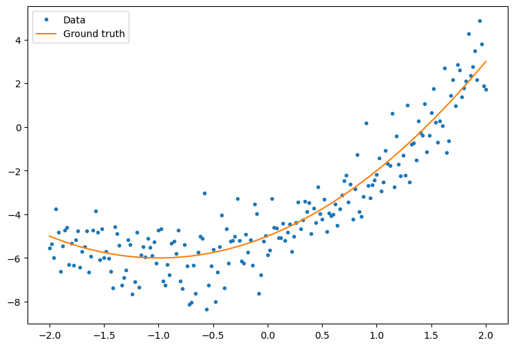
First, create some example data. This generates a cloud of points that loosely follows a quadratic curve:
import matplotlib
from matplotlib import pyplot as plt

matplotlib.rcParams['figure.figsize'] = [9, 6]
x = tf.linspace(-2, 2, 201)
x = tf.cast(x, tf.float32)

def f(x):
  y = x**2 + 2*x - 5
  return y

y = f(x) + tf.random.normal(shape=[201])

plt.plot(x.numpy(), y.numpy(), '.', label='Data')
plt.plot(x, f(x), label='Ground truth')
plt.legend();
Create a quadratic model with randomly initialized weights and a bias:
class Model(tf.Module):

  def __init__(self):
    # Randomly generate weight and bias terms
    rand_init = tf.random.uniform(shape=[3], minval=0., maxval=5., seed=22)
    # Initialize model parameters
    self.w_q = tf.Variable(rand_init[0])
    self.w_l = tf.Variable(rand_init[1])
    self.b = tf.Variable(rand_init[2])

  @tf.function
  def __call__(self, x):
    # Quadratic Model : quadratic_weight * x^2 + linear_weight * x + bias
    return self.w_q * (x**2) + self.w_l * x + self.b
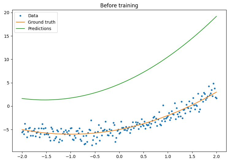
First, observe your model's performance before training:
quad_model = Model()
def plot_preds(x, y, f, model, title):
  plt.figure()
  plt.plot(x, y, '.', label='Data')
  plt.plot(x, f(x), label='Ground truth')
  plt.plot(x, model(x), label='Predictions')
  plt.title(title)
  plt.legend()
plot_preds(x, y, f, quad_model, 'Before training')
Now, define a loss for your model:
Given that this model is intended to predict continuous values, the mean squared error (MSE) is a good choice for the loss function. Given a vector of predictions, \(\hat{y}\), and a vector of true targets, \(y\), the MSE is defined as the mean of the squared differences between the predicted values and the ground truth.
\(MSE = \frac{1}{m}\sum_{i=1}^{m}(\hat{y}_i -y_i)^2\)
def mse_loss(y_pred, y):
  return tf.reduce_mean(tf.square(y_pred - y))
Write a basic training loop for the model. The loop will make use of the MSE loss function and its gradients with respect to the input in order to iteratively update the model's parameters. Using mini-batches for training provides both memory efficiency and faster convergence. The tf.data.Dataset API has useful functions for batching and shuffling.
batch_size = 32
dataset = tf.data.Dataset.from_tensor_slices((x, y))
dataset = dataset.shuffle(buffer_size=x.shape[0]).batch(batch_size)
# Set training parameters
epochs = 100
learning_rate = 0.01
losses = []
# Format training loop
for epoch in range(epochs):
for x_batch, y_batch in dataset:
with tf.GradientTape() as tape:
batch_loss = mse_loss(quad_model(x_batch), y_batch)
# Update parameters with respect to the gradient calculations
grads = tape.gradient(batch_loss, quad_model.variables)
for g,v in zip(grads, quad_model.variables):
v.assign_sub(learning_rate*g)
# Keep track of model loss per epoch
loss = mse_loss(quad_model(x), y)
losses.append(loss)
if epoch % 10 == 0:
print(f'Mean squared error for step {epoch}: {loss.numpy():0.3f}')
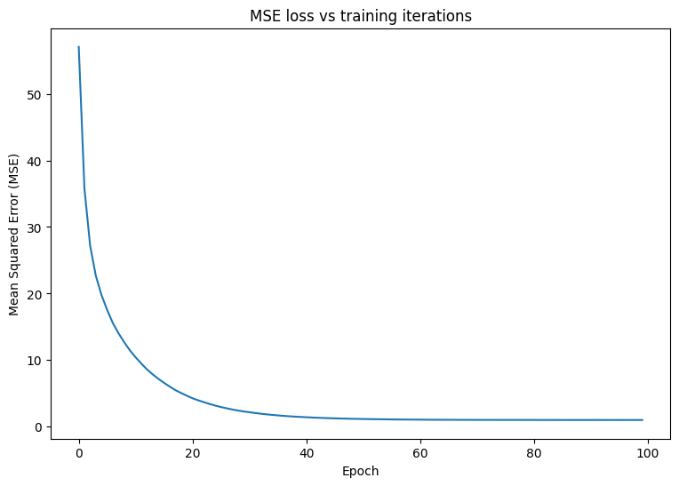
# Plot model results
print("\n")
plt.plot(range(epochs), losses)
plt.xlabel("Epoch")
plt.ylabel("Mean Squared Error (MSE)")
plt.title('MSE loss vs training iterations');
Mean squared error for step 0: 57.050
Mean squared error for step 10: 10.417
Mean squared error for step 20: 4.270
Mean squared error for step 30: 2.171
Mean squared error for step 40: 1.429
Mean squared error for step 50: 1.162
Mean squared error for step 60: 1.062
Mean squared error for step 70: 1.027
Mean squared error for step 80: 1.017
Mean squared error for step 90: 1.014
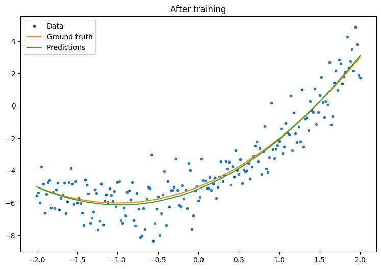
Now, observe your model's performance after training:
plot_preds(x, y, f, quad_model, 'After training')
That's working, but remember that implementations of common training utilities are available in the tf.keras module. So, consider using those before writing your own. To start with, the Model.compile and Model.fit methods implement a training loop for you:
Begin by creating a Sequential Model in Keras using tf.keras.Sequential. One of the simplest Keras layers is the dense layer, which can be instantiated with tf.keras.layers.Dense. The dense layer is able to learn multidimensional linear relationships of the form \(\mathrm{Y} = \mathrm{W}\mathrm{X} + \vec{b}\). In order to learn a nonlinear equation of the form, \(w_1x^2 + w_2x + b\), the dense layer's input should be a data matrix with \(x^2\) and \(x\) as features. The lambda layer, tf.keras.layers.Lambda, can be used to perform this stacking transformation.
new_model = tf.keras.Sequential([
    tf.keras.layers.Lambda(lambda x: tf.stack([x, x**2], axis=1)),
    tf.keras.layers.Dense(units=1, kernel_initializer=tf.random.normal)])
new_model.compile(
    loss=tf.keras.losses.MSE,
    optimizer=tf.keras.optimizers.SGD(learning_rate=0.01))

history = new_model.fit(x, y,
                        epochs=100,
                        batch_size=32,
                        verbose=0)

new_model.save('./my_new_model.keras')
WARNING: All log messages before absl::InitializeLog() is called are written to STDERR
I0000 00:00:1727918680.462363   10695 service.cc:146] XLA service 0x7f51a0006eb0 initialized for platform CUDA (this does not guarantee that XLA will be used). Devices:
I0000 00:00:1727918680.462397   10695 service.cc:154]   StreamExecutor device (0): Tesla T4, Compute Capability 7.5
I0000 00:00:1727918680.462401   10695 service.cc:154]   StreamExecutor device (1): Tesla T4, Compute Capability 7.5
I0000 00:00:1727918680.462404   10695 service.cc:154]   StreamExecutor device (2): Tesla T4, Compute Capability 7.5
I0000 00:00:1727918680.462407   10695 service.cc:154]   StreamExecutor device (3): Tesla T4, Compute Capability 7.5
I0000 00:00:1727918680.790826   10695 device_compiler.h:188] Compiled cluster using XLA!  This line is logged at most once for the lifetime of the process.
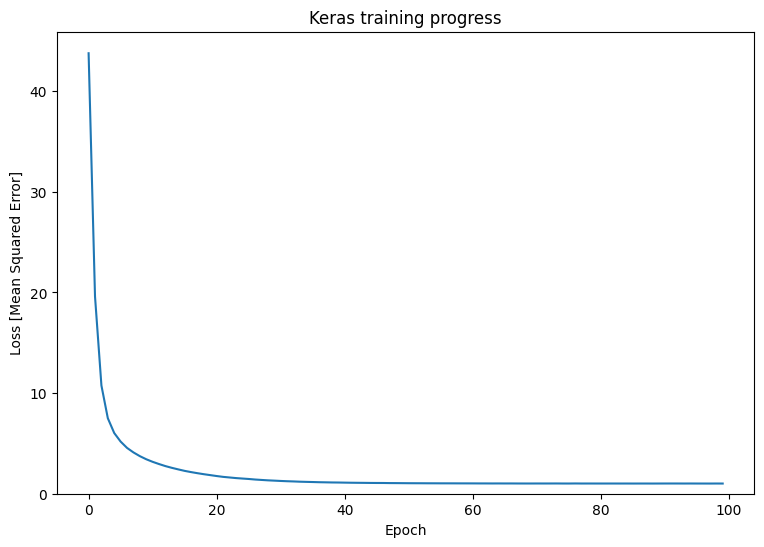
Observe your Keras model's performance after training:
plt.plot(history.history['loss'])
plt.xlabel('Epoch')
plt.ylim([0, max(plt.ylim())])
plt.ylabel('Loss [Mean Squared Error]')
plt.title('Keras training progress');
plot_preds(x, y, f, new_model, 'After Training: Keras')
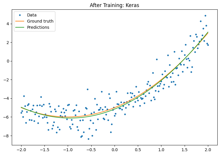
Refer to Basic training loops and the Keras guide for more details.