
|
|
|
 View on GitHub View on GitHub
|
|
|
The CORD-19 Swivel text embedding module from TF-Hub (https://tfhub.dev/tensorflow/cord-19/swivel-128d/3) was built to support researchers analyzing natural languages text related to COVID-19. These embeddings were trained on the titles, authors, abstracts, body texts, and reference titles of articles in the CORD-19 dataset.
In this colab we will:
- Analyze semantically similar words in the embedding space
- Train a classifier on the SciCite dataset using the CORD-19 embeddings
Setup
import functools
import itertools
import matplotlib.pyplot as plt
import numpy as np
import seaborn as sns
import pandas as pd

import tensorflow as tf

import tensorflow_datasets as tfds
import tensorflow_hub as hub

from tqdm import trange
2023-10-09 22:29:39.063949: E tensorflow/compiler/xla/stream_executor/cuda/cuda_dnn.cc:9342] Unable to register cuDNN factory: Attempting to register factory for plugin cuDNN when one has already been registered
2023-10-09 22:29:39.064004: E tensorflow/compiler/xla/stream_executor/cuda/cuda_fft.cc:609] Unable to register cuFFT factory: Attempting to register factory for plugin cuFFT when one has already been registered
2023-10-09 22:29:39.064046: E tensorflow/compiler/xla/stream_executor/cuda/cuda_blas.cc:1518] Unable to register cuBLAS factory: Attempting to register factory for plugin cuBLAS when one has already been registered
Analyze the embeddings
Let's start off by analyzing the embedding by calculating and plotting a correlation matrix between different terms. If the embedding learned to successfully capture the meaning of different words, the embedding vectors of semantically similar words should be close together. Let's take a look at some COVID-19 related terms.
# Use the inner product between two embedding vectors as the similarity measure
def plot_correlation(labels, features):
  corr = np.inner(features, features)
  corr /= np.max(corr)
  sns.heatmap(corr, xticklabels=labels, yticklabels=labels)

# Generate embeddings for some terms
queries = [
  # Related viruses
  'coronavirus', 'SARS', 'MERS',
  # Regions
  'Italy', 'Spain', 'Europe',
  # Symptoms
  'cough', 'fever', 'throat'
]

module = hub.load('https://tfhub.dev/tensorflow/cord-19/swivel-128d/3')
embeddings = module(queries)

plot_correlation(queries, embeddings)
2023-10-09 22:29:44.568345: E tensorflow/compiler/xla/stream_executor/cuda/cuda_driver.cc:268] failed call to cuInit: CUDA_ERROR_NO_DEVICE: no CUDA-capable device is detected
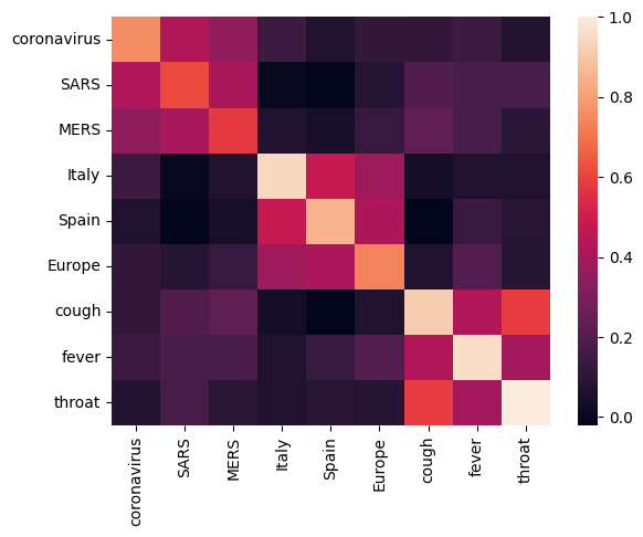
We can see that the embedding successfully captured the meaning of the different terms. Each word is similar to the other words of its cluster (i.e. "coronavirus" highly correlates with "SARS" and "MERS"), while they are different from terms of other clusters (i.e. the similarity between "SARS" and "Spain" is close to 0).
Now let's see how we can use these embeddings to solve a specific task.
SciCite: Citation Intent Classification
This section shows how one can use the embedding for downstream tasks such as text classification. We'll use the SciCite dataset from TensorFlow Datasets to classify citation intents in academic papers. Given a sentence with a citation from an academic paper, classify whether the main intent of the citation is as background information, use of methods, or comparing results.
builder = tfds.builder(name='scicite')
builder.download_and_prepare()
train_data, validation_data, test_data = builder.as_dataset(
    split=('train', 'validation', 'test'),
    as_supervised=True)
Let's take a look at a few labeled examples from the training set
NUM_EXAMPLES =   10

TEXT_FEATURE_NAME = builder.info.supervised_keys[0]
LABEL_NAME = builder.info.supervised_keys[1]

def label2str(numeric_label):
  m = builder.info.features[LABEL_NAME].names
  return m[numeric_label]

data = next(iter(train_data.batch(NUM_EXAMPLES)))


pd.DataFrame({
    TEXT_FEATURE_NAME: [ex.numpy().decode('utf8') for ex in data[0]],
    LABEL_NAME: [label2str(x) for x in data[1]]
})
Training a citaton intent classifier
We'll train a classifier on the SciCite dataset using Keras. Let's build a model which use the CORD-19 embeddings with a classification layer on top.
Hyperparameters
EMBEDDING = 'https://tfhub.dev/tensorflow/cord-19/swivel-128d/3'
TRAINABLE_MODULE = False

hub_layer = hub.KerasLayer(EMBEDDING, input_shape=[],
                           dtype=tf.string, trainable=TRAINABLE_MODULE)

model = tf.keras.Sequential()
model.add(hub_layer)
model.add(tf.keras.layers.Dense(3))
model.summary()
model.compile(optimizer='adam',
              loss=tf.keras.losses.SparseCategoricalCrossentropy(from_logits=True),
              metrics=['accuracy'])
Model: "sequential"
_________________________________________________________________
 Layer (type)                Output Shape              Param #
=================================================================
 keras_layer (KerasLayer)    (None, 128)               17301632

 dense (Dense)               (None, 3)                 387

=================================================================
Total params: 17302019 (132.00 MB)
Trainable params: 387 (1.51 KB)
Non-trainable params: 17301632 (132.00 MB)
_________________________________________________________________
Train and evaluate the model
Let's train and evaluate the model to see the performance on the SciCite task
EPOCHS = 35
BATCH_SIZE = 32

history = model.fit(train_data.shuffle(10000).batch(BATCH_SIZE),
                    epochs=EPOCHS,
                    validation_data=validation_data.batch(BATCH_SIZE),
                    verbose=1)
Epoch 1/35
257/257 [==============================] - 2s 4ms/step - loss: 0.8391 - accuracy: 0.6421 - val_loss: 0.7495 - val_accuracy: 0.7020
Epoch 2/35
257/257 [==============================] - 1s 3ms/step - loss: 0.6784 - accuracy: 0.7282 - val_loss: 0.6634 - val_accuracy: 0.7380
Epoch 3/35
257/257 [==============================] - 1s 3ms/step - loss: 0.6175 - accuracy: 0.7562 - val_loss: 0.6269 - val_accuracy: 0.7478
Epoch 4/35
257/257 [==============================] - 1s 3ms/step - loss: 0.5858 - accuracy: 0.7706 - val_loss: 0.6035 - val_accuracy: 0.7533
Epoch 5/35
257/257 [==============================] - 1s 3ms/step - loss: 0.5674 - accuracy: 0.7780 - val_loss: 0.5914 - val_accuracy: 0.7576
Epoch 6/35
257/257 [==============================] - 1s 3ms/step - loss: 0.5553 - accuracy: 0.7817 - val_loss: 0.5822 - val_accuracy: 0.7653
Epoch 7/35
257/257 [==============================] - 1s 3ms/step - loss: 0.5464 - accuracy: 0.7847 - val_loss: 0.5784 - val_accuracy: 0.7609
Epoch 8/35
257/257 [==============================] - 1s 3ms/step - loss: 0.5399 - accuracy: 0.7872 - val_loss: 0.5723 - val_accuracy: 0.7707
Epoch 9/35
257/257 [==============================] - 1s 3ms/step - loss: 0.5352 - accuracy: 0.7906 - val_loss: 0.5690 - val_accuracy: 0.7707
Epoch 10/35
257/257 [==============================] - 1s 3ms/step - loss: 0.5303 - accuracy: 0.7924 - val_loss: 0.5630 - val_accuracy: 0.7806
Epoch 11/35
257/257 [==============================] - 1s 3ms/step - loss: 0.5268 - accuracy: 0.7939 - val_loss: 0.5610 - val_accuracy: 0.7773
Epoch 12/35
257/257 [==============================] - 1s 3ms/step - loss: 0.5236 - accuracy: 0.7929 - val_loss: 0.5601 - val_accuracy: 0.7762
Epoch 13/35
257/257 [==============================] - 1s 3ms/step - loss: 0.5213 - accuracy: 0.7952 - val_loss: 0.5586 - val_accuracy: 0.7773
Epoch 14/35
257/257 [==============================] - 1s 3ms/step - loss: 0.5188 - accuracy: 0.7959 - val_loss: 0.5560 - val_accuracy: 0.7751
Epoch 15/35
257/257 [==============================] - 1s 3ms/step - loss: 0.5169 - accuracy: 0.7963 - val_loss: 0.5566 - val_accuracy: 0.7817
Epoch 16/35
257/257 [==============================] - 1s 3ms/step - loss: 0.5150 - accuracy: 0.7950 - val_loss: 0.5521 - val_accuracy: 0.7795
Epoch 17/35
257/257 [==============================] - 1s 3ms/step - loss: 0.5136 - accuracy: 0.7974 - val_loss: 0.5551 - val_accuracy: 0.7795
Epoch 18/35
257/257 [==============================] - 1s 3ms/step - loss: 0.5122 - accuracy: 0.7966 - val_loss: 0.5490 - val_accuracy: 0.7795
Epoch 19/35
257/257 [==============================] - 1s 3ms/step - loss: 0.5106 - accuracy: 0.7973 - val_loss: 0.5508 - val_accuracy: 0.7849
Epoch 20/35
257/257 [==============================] - 1s 3ms/step - loss: 0.5097 - accuracy: 0.7974 - val_loss: 0.5503 - val_accuracy: 0.7806
Epoch 21/35
257/257 [==============================] - 1s 3ms/step - loss: 0.5086 - accuracy: 0.7981 - val_loss: 0.5467 - val_accuracy: 0.7817
Epoch 22/35
257/257 [==============================] - 1s 3ms/step - loss: 0.5072 - accuracy: 0.8003 - val_loss: 0.5518 - val_accuracy: 0.7838
Epoch 23/35
257/257 [==============================] - 1s 3ms/step - loss: 0.5066 - accuracy: 0.7994 - val_loss: 0.5485 - val_accuracy: 0.7871
Epoch 24/35
257/257 [==============================] - 1s 3ms/step - loss: 0.5060 - accuracy: 0.7991 - val_loss: 0.5477 - val_accuracy: 0.7849
Epoch 25/35
257/257 [==============================] - 1s 3ms/step - loss: 0.5049 - accuracy: 0.8003 - val_loss: 0.5481 - val_accuracy: 0.7849
Epoch 26/35
257/257 [==============================] - 1s 3ms/step - loss: 0.5046 - accuracy: 0.7985 - val_loss: 0.5465 - val_accuracy: 0.7871
Epoch 27/35
257/257 [==============================] - 1s 3ms/step - loss: 0.5035 - accuracy: 0.7999 - val_loss: 0.5457 - val_accuracy: 0.7828
Epoch 28/35
257/257 [==============================] - 1s 3ms/step - loss: 0.5030 - accuracy: 0.8011 - val_loss: 0.5474 - val_accuracy: 0.7838
Epoch 29/35
257/257 [==============================] - 1s 3ms/step - loss: 0.5025 - accuracy: 0.8007 - val_loss: 0.5484 - val_accuracy: 0.7871
Epoch 30/35
257/257 [==============================] - 1s 3ms/step - loss: 0.5016 - accuracy: 0.8023 - val_loss: 0.5440 - val_accuracy: 0.7904
Epoch 31/35
257/257 [==============================] - 1s 3ms/step - loss: 0.5011 - accuracy: 0.8003 - val_loss: 0.5487 - val_accuracy: 0.7849
Epoch 32/35
257/257 [==============================] - 1s 3ms/step - loss: 0.5011 - accuracy: 0.8012 - val_loss: 0.5451 - val_accuracy: 0.7882
Epoch 33/35
257/257 [==============================] - 1s 3ms/step - loss: 0.5005 - accuracy: 0.8011 - val_loss: 0.5464 - val_accuracy: 0.7882
Epoch 34/35
257/257 [==============================] - 1s 3ms/step - loss: 0.5000 - accuracy: 0.8014 - val_loss: 0.5486 - val_accuracy: 0.7871
Epoch 35/35
257/257 [==============================] - 1s 3ms/step - loss: 0.4995 - accuracy: 0.8006 - val_loss: 0.5485 - val_accuracy: 0.7871
from matplotlib import pyplot as plt
def display_training_curves(training, validation, title, subplot):
  if subplot%10==1: # set up the subplots on the first call
    plt.subplots(figsize=(10,10), facecolor='#F0F0F0')
    plt.tight_layout()
  ax = plt.subplot(subplot)
  ax.set_facecolor('#F8F8F8')
  ax.plot(training)
  ax.plot(validation)
  ax.set_title('model '+ title)
  ax.set_ylabel(title)
  ax.set_xlabel('epoch')
  ax.legend(['train', 'valid.'])
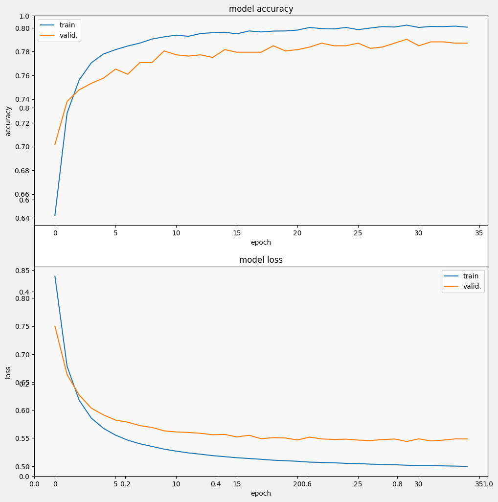
display_training_curves(history.history['accuracy'], history.history['val_accuracy'], 'accuracy', 211)
display_training_curves(history.history['loss'], history.history['val_loss'], 'loss', 212)
Evaluate the model
And let's see how the model performs. Two values will be returned. Loss (a number which represents our error, lower values are better), and accuracy.
results = model.evaluate(test_data.batch(512), verbose=2)

for name, value in zip(model.metrics_names, results):
  print('%s: %.3f' % (name, value))
4/4 - 0s - loss: 0.5406 - accuracy: 0.7805 - 293ms/epoch - 73ms/step
loss: 0.541
accuracy: 0.781
We can see that the loss quickly decreases while especially the accuracy rapidly increases. Let's plot some examples to check how the prediction relates to the true labels:
prediction_dataset = next(iter(test_data.batch(20)))

prediction_texts = [ex.numpy().decode('utf8') for ex in prediction_dataset[0]]
prediction_labels = [label2str(x) for x in prediction_dataset[1]]

predictions = [
    label2str(x) for x in np.argmax(model.predict(prediction_texts), axis=-1)]


pd.DataFrame({
    TEXT_FEATURE_NAME: prediction_texts,
    LABEL_NAME: prediction_labels,
    'prediction': predictions
})
1/1 [==============================] - 0s 122ms/step
We can see that for this random sample, the model predicts the correct label most of the times, indicating that it can embed scientific sentences pretty well.
What's next?
Now that you've gotten to know a bit more about the CORD-19 Swivel embeddings from TF-Hub, we encourage you to participate in the CORD-19 Kaggle competition to contribute to gaining scientific insights from COVID-19 related academic texts.
- Participate in the CORD-19 Kaggle Challenge
- Learn more about the COVID-19 Open Research Dataset (CORD-19)
- See documentation and more about the TF-Hub embeddings at https://tfhub.dev/tensorflow/cord-19/swivel-128d/3
- Explore the CORD-19 embedding space with the TensorFlow Embedding Projector