
|
|
|
 View on GitHub View on GitHub
|
|
|
TF-Hub is a platform to share machine learning expertise packaged in reusable resources, notably pre-trained modules. In this tutorial, we will use a TF-Hub text embedding module to train a simple sentiment classifier with a reasonable baseline accuracy. We will then submit the predictions to Kaggle.
For more detailed tutorial on text classification with TF-Hub and further steps for improving the accuracy, take a look at Text classification with TF-Hub.
Setup
pip install -q kaggleimport tensorflow as tf
import tensorflow_hub as hub
import matplotlib.pyplot as plt
import numpy as np
import pandas as pd
import seaborn as sns
import zipfile
from sklearn import model_selection
Since this tutorial will be using a dataset from Kaggle, it requires creating an API Token for your Kaggle account, and uploading it to the Colab environment.
import os
import pathlib

# Upload the API token.
def get_kaggle():
  try:
    import kaggle
    return kaggle
  except OSError:
    pass

  token_file = pathlib.Path("~/.kaggle/kaggle.json").expanduser()
  token_file.parent.mkdir(exist_ok=True, parents=True)

  try:
    from google.colab import files
  except ImportError:
    raise ValueError("Could not find kaggle token.")

  uploaded = files.upload()
  token_content = uploaded.get('kaggle.json', None)
  if token_content:
    token_file.write_bytes(token_content)
    token_file.chmod(0o600)
  else:
    raise ValueError('Need a file named "kaggle.json"')

  import kaggle
  return kaggle


kaggle = get_kaggle()
Getting started
Data
We will try to solve the Sentiment Analysis on Movie Reviews task from Kaggle. The dataset consists of syntactic subphrases of the Rotten Tomatoes movie reviews. The task is to label the phrases as negative or positive on the scale from 1 to 5.
You must accept the competition rules before you can use the API to download the data.
SENTIMENT_LABELS = [
    "negative", "somewhat negative", "neutral", "somewhat positive", "positive"
]

# Add a column with readable values representing the sentiment.
def add_readable_labels_column(df, sentiment_value_column):
  df["SentimentLabel"] = df[sentiment_value_column].replace(
      range(5), SENTIMENT_LABELS)

# Download data from Kaggle and create a DataFrame.
def load_data_from_zip(path):
  with zipfile.ZipFile(path, "r") as zip_ref:
    name = zip_ref.namelist()[0]
    with zip_ref.open(name) as zf:
      return pd.read_csv(zf, sep="\t", index_col=0)


# The data does not come with a validation set so we'll create one from the
# training set.
def get_data(competition, train_file, test_file, validation_set_ratio=0.1):
  data_path = pathlib.Path("data")
  kaggle.api.competition_download_files(competition, data_path)
  competition_path = (data_path/competition)
  competition_path.mkdir(exist_ok=True, parents=True)
  competition_zip_path = competition_path.with_suffix(".zip")

  with zipfile.ZipFile(competition_zip_path, "r") as zip_ref:
    zip_ref.extractall(competition_path)

  train_df = load_data_from_zip(competition_path/train_file)
  test_df = load_data_from_zip(competition_path/test_file)

  # Add a human readable label.
  add_readable_labels_column(train_df, "Sentiment")

  # We split by sentence ids, because we don't want to have phrases belonging
  # to the same sentence in both training and validation set.
  train_indices, validation_indices = model_selection.train_test_split(
      np.unique(train_df["SentenceId"]),
      test_size=validation_set_ratio,
      random_state=0)

  validation_df = train_df[train_df["SentenceId"].isin(validation_indices)]
  train_df = train_df[train_df["SentenceId"].isin(train_indices)]
  print("Split the training data into %d training and %d validation examples." %
        (len(train_df), len(validation_df)))

  return train_df, validation_df, test_df


train_df, validation_df, test_df = get_data(
    "sentiment-analysis-on-movie-reviews",
    "train.tsv.zip", "test.tsv.zip")
Split the training data into 140315 training and 15745 validation examples.
train_df.head(20)
Training an Model
class MyModel(tf.keras.Model):
  def __init__(self, hub_url):
    super().__init__()
    self.hub_url = hub_url
    self.embed = hub.load(self.hub_url).signatures['default']
    self.sequential = tf.keras.Sequential([
      tf.keras.layers.Dense(500),
      tf.keras.layers.Dense(100),
      tf.keras.layers.Dense(5),
    ])

  def call(self, inputs):
    phrases = inputs['Phrase'][:,0]
    embedding = 5*self.embed(phrases)['default']
    return self.sequential(embedding)

  def get_config(self):
    return {"hub_url":self.hub_url}
model = MyModel("https://tfhub.dev/google/nnlm-en-dim128/1")
model.compile(
    loss = tf.losses.SparseCategoricalCrossentropy(from_logits=True),
    optimizer=tf.optimizers.Adam(),
    metrics = [tf.keras.metrics.SparseCategoricalAccuracy(name="accuracy")])
2024-03-09 13:31:20.808764: E external/local_xla/xla/stream_executor/cuda/cuda_driver.cc:282] failed call to cuInit: CUDA_ERROR_NO_DEVICE: no CUDA-capable device is detected
history = model.fit(x=dict(train_df), y=train_df['Sentiment'],
          validation_data=(dict(validation_df), validation_df['Sentiment']),
          epochs = 25)
Epoch 1/25
4385/4385 ━━━━━━━━━━━━━━━━━━━━ 17s 4ms/step - accuracy: 0.5711 - loss: 1.0662 - val_accuracy: 0.5910 - val_loss: 1.0030
Epoch 2/25
4385/4385 ━━━━━━━━━━━━━━━━━━━━ 16s 4ms/step - accuracy: 0.5939 - loss: 1.0012 - val_accuracy: 0.5965 - val_loss: 0.9947
Epoch 3/25
4385/4385 ━━━━━━━━━━━━━━━━━━━━ 16s 4ms/step - accuracy: 0.5967 - loss: 0.9949 - val_accuracy: 0.5940 - val_loss: 0.9910
Epoch 4/25
4385/4385 ━━━━━━━━━━━━━━━━━━━━ 16s 4ms/step - accuracy: 0.5978 - loss: 0.9944 - val_accuracy: 0.5910 - val_loss: 0.9921
Epoch 5/25
4385/4385 ━━━━━━━━━━━━━━━━━━━━ 16s 4ms/step - accuracy: 0.5959 - loss: 0.9923 - val_accuracy: 0.5906 - val_loss: 0.9898
Epoch 6/25
4385/4385 ━━━━━━━━━━━━━━━━━━━━ 16s 4ms/step - accuracy: 0.5984 - loss: 0.9890 - val_accuracy: 0.5950 - val_loss: 0.9861
Epoch 7/25
4385/4385 ━━━━━━━━━━━━━━━━━━━━ 16s 4ms/step - accuracy: 0.5967 - loss: 0.9887 - val_accuracy: 0.5883 - val_loss: 0.9970
Epoch 8/25
4385/4385 ━━━━━━━━━━━━━━━━━━━━ 16s 4ms/step - accuracy: 0.5968 - loss: 0.9893 - val_accuracy: 0.6026 - val_loss: 0.9858
Epoch 9/25
4385/4385 ━━━━━━━━━━━━━━━━━━━━ 16s 4ms/step - accuracy: 0.5982 - loss: 0.9883 - val_accuracy: 0.5940 - val_loss: 0.9888
Epoch 10/25
4385/4385 ━━━━━━━━━━━━━━━━━━━━ 16s 4ms/step - accuracy: 0.5986 - loss: 0.9910 - val_accuracy: 0.6008 - val_loss: 0.9815
Epoch 11/25
4385/4385 ━━━━━━━━━━━━━━━━━━━━ 16s 4ms/step - accuracy: 0.5988 - loss: 0.9869 - val_accuracy: 0.5960 - val_loss: 0.9871
Epoch 12/25
4385/4385 ━━━━━━━━━━━━━━━━━━━━ 16s 4ms/step - accuracy: 0.6008 - loss: 0.9863 - val_accuracy: 0.5942 - val_loss: 0.9863
Epoch 13/25
4385/4385 ━━━━━━━━━━━━━━━━━━━━ 16s 4ms/step - accuracy: 0.5996 - loss: 0.9878 - val_accuracy: 0.5990 - val_loss: 0.9886
Epoch 14/25
4385/4385 ━━━━━━━━━━━━━━━━━━━━ 16s 4ms/step - accuracy: 0.6022 - loss: 0.9852 - val_accuracy: 0.5969 - val_loss: 0.9831
Epoch 15/25
4385/4385 ━━━━━━━━━━━━━━━━━━━━ 16s 4ms/step - accuracy: 0.5960 - loss: 0.9910 - val_accuracy: 0.5971 - val_loss: 0.9851
Epoch 16/25
4385/4385 ━━━━━━━━━━━━━━━━━━━━ 16s 4ms/step - accuracy: 0.5991 - loss: 0.9887 - val_accuracy: 0.6022 - val_loss: 0.9840
Epoch 17/25
4385/4385 ━━━━━━━━━━━━━━━━━━━━ 16s 4ms/step - accuracy: 0.6007 - loss: 0.9856 - val_accuracy: 0.5987 - val_loss: 0.9832
Epoch 18/25
4385/4385 ━━━━━━━━━━━━━━━━━━━━ 16s 4ms/step - accuracy: 0.6010 - loss: 0.9873 - val_accuracy: 0.5994 - val_loss: 0.9848
Epoch 19/25
4385/4385 ━━━━━━━━━━━━━━━━━━━━ 16s 4ms/step - accuracy: 0.5986 - loss: 0.9877 - val_accuracy: 0.5969 - val_loss: 0.9938
Epoch 20/25
4385/4385 ━━━━━━━━━━━━━━━━━━━━ 16s 4ms/step - accuracy: 0.6006 - loss: 0.9857 - val_accuracy: 0.5914 - val_loss: 0.9933
Epoch 21/25
4385/4385 ━━━━━━━━━━━━━━━━━━━━ 16s 4ms/step - accuracy: 0.5986 - loss: 0.9870 - val_accuracy: 0.5956 - val_loss: 0.9882
Epoch 22/25
4385/4385 ━━━━━━━━━━━━━━━━━━━━ 16s 4ms/step - accuracy: 0.5997 - loss: 0.9866 - val_accuracy: 0.5966 - val_loss: 0.9882
Epoch 23/25
4385/4385 ━━━━━━━━━━━━━━━━━━━━ 16s 4ms/step - accuracy: 0.5989 - loss: 0.9837 - val_accuracy: 0.5910 - val_loss: 0.9869
Epoch 24/25
4385/4385 ━━━━━━━━━━━━━━━━━━━━ 16s 4ms/step - accuracy: 0.5981 - loss: 0.9872 - val_accuracy: 0.6011 - val_loss: 0.9812
Epoch 25/25
4385/4385 ━━━━━━━━━━━━━━━━━━━━ 16s 4ms/step - accuracy: 0.6018 - loss: 0.9834 - val_accuracy: 0.5976 - val_loss: 0.9854
Prediction
Run predictions for the validation set and training set.
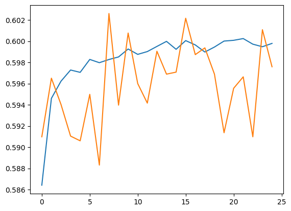
plt.plot(history.history['accuracy'])
plt.plot(history.history['val_accuracy'])
[<matplotlib.lines.Line2D at 0x7fcfc99b88e0>]
train_eval_result = model.evaluate(dict(train_df), train_df['Sentiment'])
validation_eval_result = model.evaluate(dict(validation_df), validation_df['Sentiment'])

print(f"Training set accuracy: {train_eval_result[1]}")
print(f"Validation set accuracy: {validation_eval_result[1]}")
4385/4385 ━━━━━━━━━━━━━━━━━━━━ 16s 4ms/step - accuracy: 0.6212 - loss: 0.9463
493/493 ━━━━━━━━━━━━━━━━━━━━ 1s 1ms/step - accuracy: 0.6105 - loss: 0.9561
Training set accuracy: 0.6025798916816711
Validation set accuracy: 0.5975865125656128
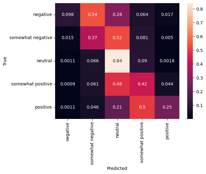
Confusion matrix
Another very interesting statistic, especially for multiclass problems, is the confusion matrix. The confusion matrix allows visualization of the proportion of correctly and incorrectly labelled examples. We can easily see how much our classifier is biased and whether the distribution of labels makes sense. Ideally the largest fraction of predictions should be distributed along the diagonal.
predictions = model.predict(dict(validation_df))
predictions = tf.argmax(predictions, axis=-1)
predictions
493/493 ━━━━━━━━━━━━━━━━━━━━ 1s 1ms/step
<tf.Tensor: shape=(15745,), dtype=int64, numpy=array([1, 1, 2, ..., 2, 2, 2])>
cm = tf.math.confusion_matrix(validation_df['Sentiment'], predictions)
cm = cm/cm.numpy().sum(axis=1)[:, tf.newaxis]
sns.heatmap(
    cm, annot=True,
    xticklabels=SENTIMENT_LABELS,
    yticklabels=SENTIMENT_LABELS)
plt.xlabel("Predicted")
plt.ylabel("True")
Text(50.72222222222221, 0.5, 'True')
We can easily submit the predictions back to Kaggle by pasting the following code to a code cell and executing it:
test_predictions = model.predict(dict(test_df))
test_predictions = np.argmax(test_predictions, axis=-1)

result_df = test_df.copy()

result_df["Predictions"] = test_predictions

result_df.to_csv(
    "predictions.csv",
    columns=["Predictions"],
    header=["Sentiment"])
kaggle.api.competition_submit("predictions.csv", "Submitted from Colab",
                              "sentiment-analysis-on-movie-reviews")
After submitting, check the leaderboard to see how you did.