TensorFlow Probability のツアー

TensorFlow.org で表示

Google Colab で実行

GitHubでソースを表示

ノートブックをダウンロード

この Colab では、TensorFlow Probability の基本的な機能の一部を紹介します。

依存関係と前提条件

Import

from pprint import pprint
import matplotlib.pyplot as plt
import numpy as np
import seaborn as sns

import tensorflow.compat.v2 as tf
tf.enable_v2_behavior()

import tensorflow_probability as tfp

sns.reset_defaults()
sns.set_context(context='talk',font_scale=0.7)
plt.rcParams['image.cmap'] = 'viridis'

%matplotlib inline

tfd = tfp.distributions
tfb = tfp.bijectors

Utils

def print_subclasses_from_module(module, base_class, maxwidth=80):
  import functools, inspect, sys
  subclasses = [name for name, obj in inspect.getmembers(module)
                if inspect.isclass(obj) and issubclass(obj, base_class)]
  def red(acc, x):
    if not acc or len(acc[-1]) + len(x) + 2 > maxwidth:
      acc.append(x)
    else:
      acc[-1] += ", " + x
    return acc
  print('\n'.join(functools.reduce(red, subclasses, [])))

概要

• TensorFlow
• TensorFlow Probability
  • 分布
  • Bijectors
  • MCMC
  • ... その他

はじめに: TensorFlow

TensorFlow は科学計算ライブラリです。

次の項目をサポートしています。

• 多数の数学演算
• 効率的なベクトル計算
• 簡単なハードウェアアクセラレーション
• 自動微分

ベクトル化

• ベクトル化によって高速化することができます！
• 形状を重視していることでもあります。

mats = tf.random.uniform(shape=[1000, 10, 10])
vecs = tf.random.uniform(shape=[1000, 10, 1])

def for_loop_solve():
  return np.array(
    [tf.linalg.solve(mats[i, ...], vecs[i, ...]) for i in range(1000)])

def vectorized_solve():
  return tf.linalg.solve(mats, vecs)

# Vectorization for the win!
%timeit for_loop_solve()
%timeit vectorized_solve()

1 loops, best of 3: 2 s per loop
1000 loops, best of 3: 653 µs per loop

ハードウェアアクセラレーション

# Code can run seamlessly on a GPU, just change Colab runtime type
# in the 'Runtime' menu.
if tf.test.gpu_device_name() == '/device:GPU:0':
  print("Using a GPU")
else:
  print("Using a CPU")

Using a CPU

自動微分

a = tf.constant(np.pi)
b = tf.constant(np.e)
with tf.GradientTape() as tape:
  tape.watch([a, b])
  c = .5 * (a**2 + b**2)
grads = tape.gradient(c, [a, b])
print(grads[0])
print(grads[1])

tf.Tensor(3.1415927, shape=(), dtype=float32)
tf.Tensor(2.7182817, shape=(), dtype=float32)

TensorFlow Probability

TensorFlow Probability は TensorFlow における確率論的推論と統計分析用のライブラリです。

低レベルのモジュール式コンポーネントを通じて、モデリング、推論、および批評をサポートしています。

低レベルのビルディングブロック

• 分布
• Bijectors

高レベルのコンストラクト

• マルコフ連鎖モンテカルロ法
• 確率的レイヤー
• 構造時系列
• 一般化線形モデル
• オプティマイザー

分布

tfp.distributions.Distribution は、sample と log_prob という 2 つのコアモデルを持つクラスです。

TFP には多数の分布があります！

print_subclasses_from_module(tfp.distributions, tfp.distributions.Distribution)

Autoregressive, BatchReshape, Bates, Bernoulli, Beta, BetaBinomial, Binomial
Blockwise, Categorical, Cauchy, Chi, Chi2, CholeskyLKJ, ContinuousBernoulli
Deterministic, Dirichlet, DirichletMultinomial, Distribution, DoublesidedMaxwell
Empirical, ExpGamma, ExpRelaxedOneHotCategorical, Exponential, FiniteDiscrete
Gamma, GammaGamma, GaussianProcess, GaussianProcessRegressionModel
GeneralizedNormal, GeneralizedPareto, Geometric, Gumbel, HalfCauchy, HalfNormal
HalfStudentT, HiddenMarkovModel, Horseshoe, Independent, InverseGamma
InverseGaussian, JohnsonSU, JointDistribution, JointDistributionCoroutine
JointDistributionCoroutineAutoBatched, JointDistributionNamed
JointDistributionNamedAutoBatched, JointDistributionSequential
JointDistributionSequentialAutoBatched, Kumaraswamy, LKJ, Laplace
LinearGaussianStateSpaceModel, LogLogistic, LogNormal, Logistic, LogitNormal
Mixture, MixtureSameFamily, Moyal, Multinomial, MultivariateNormalDiag
MultivariateNormalDiagPlusLowRank, MultivariateNormalFullCovariance
MultivariateNormalLinearOperator, MultivariateNormalTriL
MultivariateStudentTLinearOperator, NegativeBinomial, Normal, OneHotCategorical
OrderedLogistic, PERT, Pareto, PixelCNN, PlackettLuce, Poisson
PoissonLogNormalQuadratureCompound, PowerSpherical, ProbitBernoulli
QuantizedDistribution, RelaxedBernoulli, RelaxedOneHotCategorical, Sample
SinhArcsinh, SphericalUniform, StudentT, StudentTProcess
TransformedDistribution, Triangular, TruncatedCauchy, TruncatedNormal, Uniform
VariationalGaussianProcess, VectorDeterministic, VonMises
VonMisesFisher, Weibull, WishartLinearOperator, WishartTriL, Zipf

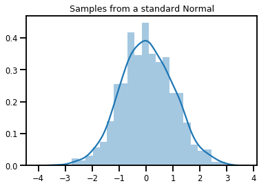
単純なスカラー変量 Distribution

# A standard normal
normal = tfd.Normal(loc=0., scale=1.)
print(normal)

tfp.distributions.Normal("Normal", batch_shape=[], event_shape=[], dtype=float32)

# Plot 1000 samples from a standard normal
samples = normal.sample(1000)
sns.distplot(samples)
plt.title("Samples from a standard Normal")
plt.show()

# Compute the log_prob of a point in the event space of `normal`
normal.log_prob(0.)

<tf.Tensor: shape=(), dtype=float32, numpy=-0.9189385>

# Compute the log_prob of a few points
normal.log_prob([-1., 0., 1.])

<tf.Tensor: shape=(3,), dtype=float32, numpy=array([-1.4189385, -0.9189385, -1.4189385], dtype=float32)>

分布と形状

Numpy ndarrays と TensorFlow Tensors には形状があります。

TensorFlow Probability Distributions には形状セマンティクスがあり、全体に同じメモリチャンク（Tensor/ndarray）が使用されている場合でも、形状を意味的に異なる部分に分割します。

• バッチ形状は、さまざまなパラメータで Distribution の集合体を示します。
• イベント形状は、Distribution のサンプルの形状を示します。

常に、バッチ形状を「左」に、イベント形状を「右」に置きます。

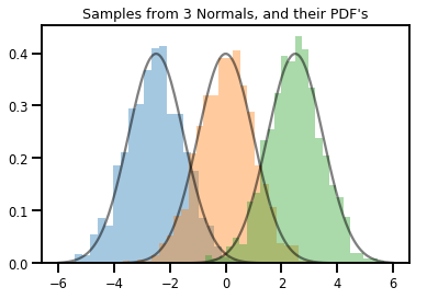
スカラー変量 Distributions のバッチ

バッチは「ベクトル化された」分布のようなもので、計算が並行して行われる独立したインスタンスです。

# Create a batch of 3 normals, and plot 1000 samples from each
normals = tfd.Normal([-2.5, 0., 2.5], 1.)  # The scale parameter broadacasts!
print("Batch shape:", normals.batch_shape)
print("Event shape:", normals.event_shape)

Batch shape: (3,)
Event shape: ()

# Samples' shapes go on the left!
samples = normals.sample(1000)
print("Shape of samples:", samples.shape)

Shape of samples: (1000, 3)

# Sample shapes can themselves be more complicated
print("Shape of samples:", normals.sample([10, 10, 10]).shape)

Shape of samples: (10, 10, 10, 3)

# A batch of normals gives a batch of log_probs.
print(normals.log_prob([-2.5, 0., 2.5]))

tf.Tensor([-0.9189385 -0.9189385 -0.9189385], shape=(3,), dtype=float32)

# The computation broadcasts, so a batch of normals applied to a scalar
# also gives a batch of log_probs.
print(normals.log_prob(0.))

tf.Tensor([-4.0439386 -0.9189385 -4.0439386], shape=(3,), dtype=float32)

# Normal numpy-like broadcasting rules apply!
xs = np.linspace(-6, 6, 200)
try:
  normals.log_prob(xs)
except Exception as e:
  print("TFP error:", e.message)

TFP error: Incompatible shapes: [200] vs. [3] [Op:SquaredDifference]

# That fails for the same reason this does:
try:
  np.zeros(200) + np.zeros(3)
except Exception as e:
  print("Numpy error:", e)

Numpy error: operands could not be broadcast together with shapes (200,) (3,)

# But this would work:
a = np.zeros([200, 1]) + np.zeros(3)
print("Broadcast shape:", a.shape)

Broadcast shape: (200, 3)

# And so will this!
xs = np.linspace(-6, 6, 200)[..., np.newaxis]
# => shape = [200, 1]

lps = normals.log_prob(xs)
print("Broadcast log_prob shape:", lps.shape)

Broadcast log_prob shape: (200, 3)

# Summarizing visually
for i in range(3):
  sns.distplot(samples[:, i], kde=False, norm_hist=True)
plt.plot(np.tile(xs, 3), normals.prob(xs), c='k', alpha=.5)
plt.title("Samples from 3 Normals, and their PDF's")
plt.show()

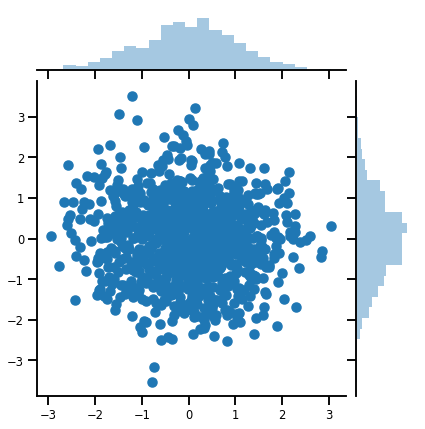
ベクトル変量 Distribution

mvn = tfd.MultivariateNormalDiag(loc=[0., 0.], scale_diag = [1., 1.])
print("Batch shape:", mvn.batch_shape)
print("Event shape:", mvn.event_shape)

Batch shape: ()
Event shape: (2,)

samples = mvn.sample(1000)
print("Samples shape:", samples.shape)

Samples shape: (1000, 2)

g = sns.jointplot(x=samples[:, 0], y=samples[:, 1], kind='scatter')
plt.show()

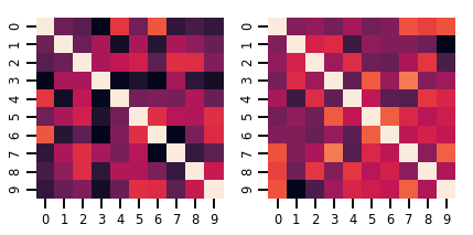
マトリクス変量 Distribution

lkj = tfd.LKJ(dimension=10, concentration=[1.5, 3.0])
print("Batch shape: ", lkj.batch_shape)
print("Event shape: ", lkj.event_shape)

Batch shape:  (2,)
Event shape:  (10, 10)

samples = lkj.sample()
print("Samples shape: ", samples.shape)

Samples shape:  (2, 10, 10)

fig, axes = plt.subplots(nrows=1, ncols=2, figsize=(6, 3))
sns.heatmap(samples[0, ...], ax=axes[0], cbar=False)
sns.heatmap(samples[1, ...], ax=axes[1], cbar=False)
fig.tight_layout()
plt.show()

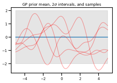
ガウス処理

kernel = tfp.math.psd_kernels.ExponentiatedQuadratic()
xs = np.linspace(-5., 5., 200).reshape([-1, 1])
gp = tfd.GaussianProcess(kernel, index_points=xs)
print("Batch shape:", gp.batch_shape)
print("Event shape:", gp.event_shape)

Batch shape: ()
Event shape: (200,)

upper, lower = gp.mean() + [2 * gp.stddev(), -2 * gp.stddev()]
plt.plot(xs, gp.mean())
plt.fill_between(xs[..., 0], upper, lower, color='k', alpha=.1)
for _ in range(5):
  plt.plot(xs, gp.sample(), c='r', alpha=.3)
plt.title(r"GP prior mean, $2\sigma$ intervals, and samples")
plt.show()

#    *** Bonus question ***
# Why do so many of these functions lie outside the 95% intervals?

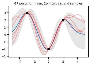
GP 回帰

# Suppose we have some observed data
obs_x = [[-3.], [0.], [2.]]  # Shape 3x1 (3 1-D vectors)
obs_y = [3., -2., 2.]        # Shape 3   (3 scalars)

gprm = tfd.GaussianProcessRegressionModel(kernel, xs, obs_x, obs_y)

upper, lower = gprm.mean() + [2 * gprm.stddev(), -2 * gprm.stddev()]
plt.plot(xs, gprm.mean())
plt.fill_between(xs[..., 0], upper, lower, color='k', alpha=.1)
for _ in range(5):
  plt.plot(xs, gprm.sample(), c='r', alpha=.3)
plt.scatter(obs_x, obs_y, c='k', zorder=3)
plt.title(r"GP posterior mean, $2\sigma$ intervals, and samples")
plt.show()

Bijectors

Bijector は（ほぼ）可逆的で円滑な関数を表します。サンプルを取得して log_probs を計算する能力を維持したまま分布を変換するために使用することができます。tfp.bijectors モジュール内に存在する場合があります。

Bijector ごとに、少なくとも次の 3 つのメソッドが実装されます。

• forward
• inverse
• （少なくとも）forward_log_det_jacobian と inverse_log_det_jacobian のいずれか。

これらを材料として、分布を変換し、さらにサンプルを取得して結果の probs をログ記録することができます。

やや煩雑な数学

• \(X\) は pdf \(p(x)\) のランダム変数です。
• \(g\) は \(X\) の空間における円滑な可逆関数です。
• \(Y = g(X)\) は新しい変換済み確率変数です。
• \(p(Y=y) = p(X=g^{-1}(y)) \cdot |\nabla g^{-1}(y)|\)

キャッシング

Bijectors は前方計算と可逆計算、そして log-det-Jacobian のキャッシュも行うため、非常にコストのかかる演算を繰り返す必要がありません。

print_subclasses_from_module(tfp.bijectors, tfp.bijectors.Bijector)

AbsoluteValue, Affine, AffineLinearOperator, AffineScalar, BatchNormalization
Bijector, Blockwise, Chain, CholeskyOuterProduct, CholeskyToInvCholesky
CorrelationCholesky, Cumsum, DiscreteCosineTransform, Exp, Expm1, FFJORD
FillScaleTriL, FillTriangular, FrechetCDF, GeneralizedExtremeValueCDF
GeneralizedPareto, GompertzCDF, GumbelCDF, Identity, Inline, Invert
IteratedSigmoidCentered, KumaraswamyCDF, LambertWTail, Log, Log1p
MaskedAutoregressiveFlow, MatrixInverseTriL, MatvecLU, MoyalCDF, NormalCDF
Ordered, Pad, Permute, PowerTransform, RationalQuadraticSpline, RayleighCDF
RealNVP, Reciprocal, Reshape, Scale, ScaleMatvecDiag, ScaleMatvecLU
ScaleMatvecLinearOperator, ScaleMatvecTriL, ScaleTriL, Shift, ShiftedGompertzCDF
Sigmoid, Sinh, SinhArcsinh, SoftClip, Softfloor, SoftmaxCentered, Softplus
Softsign, Split, Square, Tanh, TransformDiagonal, Transpose, WeibullCDF

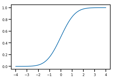
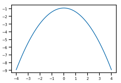
単純な Bijector

normal_cdf = tfp.bijectors.NormalCDF()
xs = np.linspace(-4., 4., 200)
plt.plot(xs, normal_cdf.forward(xs))
plt.show()

plt.plot(xs, normal_cdf.forward_log_det_jacobian(xs, event_ndims=0))
plt.show()

Bijector による Distribution の変換

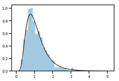
exp_bijector = tfp.bijectors.Exp()
log_normal = exp_bijector(tfd.Normal(0., .5))

samples = log_normal.sample(1000)
xs = np.linspace(1e-10, np.max(samples), 200)
sns.distplot(samples, norm_hist=True, kde=False)
plt.plot(xs, log_normal.prob(xs), c='k', alpha=.75)
plt.show()

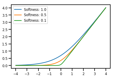
Bijectors のバッチ処理

# Create a batch of bijectors of shape [3,]
softplus = tfp.bijectors.Softplus(
  hinge_softness=[1., .5, .1])
print("Hinge softness shape:", softplus.hinge_softness.shape)

Hinge softness shape: (3,)

# For broadcasting, we want this to be shape [200, 1]
xs = np.linspace(-4., 4., 200)[..., np.newaxis]
ys = softplus.forward(xs)
print("Forward shape:", ys.shape)

Forward shape: (200, 3)

# Visualization
lines = plt.plot(np.tile(xs, 3), ys)
for line, hs in zip(lines, softplus.hinge_softness):
  line.set_label("Softness: %1.1f" % hs)
plt.legend()
plt.show()

キャッシング

# This bijector represents a matrix outer product on the forward pass,
# and a cholesky decomposition on the inverse pass. The latter costs O(N^3)!
bij = tfb.CholeskyOuterProduct()

size = 2500
# Make a big, lower-triangular matrix
big_lower_triangular = tf.eye(size)
# Squaring it gives us a positive-definite matrix
big_positive_definite = bij.forward(big_lower_triangular)

# Caching for the win!
%timeit bij.inverse(big_positive_definite)
%timeit tf.linalg.cholesky(big_positive_definite)

10000 loops, best of 3: 114 µs per loop
1 loops, best of 3: 208 ms per loop

MCMC

TFP には、ハミルトニアンモンテカルロ法など、いくつかの標準的なマルコフ連鎖モンテカルロアルゴリズムのサポートが組み込まれています。

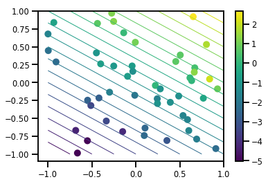
データセットを生成する

# Generate some data
def f(x, w):
  # Pad x with 1's so we can add bias via matmul
  x = tf.pad(x, [[1, 0], [0, 0]], constant_values=1)
  linop = tf.linalg.LinearOperatorFullMatrix(w[..., np.newaxis])
  result = linop.matmul(x, adjoint=True)
  return result[..., 0, :]

num_features = 2
num_examples = 50
noise_scale = .5
true_w = np.array([-1., 2., 3.])

xs = np.random.uniform(-1., 1., [num_features, num_examples])
ys = f(xs, true_w) + np.random.normal(0., noise_scale, size=num_examples)

# Visualize the data set
plt.scatter(*xs, c=ys, s=100, linewidths=0)

grid = np.meshgrid(*([np.linspace(-1, 1, 100)] * 2))
xs_grid = np.stack(grid, axis=0)
fs_grid = f(xs_grid.reshape([num_features, -1]), true_w)
fs_grid = np.reshape(fs_grid, [100, 100])
plt.colorbar()
plt.contour(xs_grid[0, ...], xs_grid[1, ...], fs_grid, 20, linewidths=1)
plt.show()

結合 log-prob 関数を定義する

同時対数確率の部分適用を形成するためにデータを閉じると、非正規化された事後確率となります。

# Define the joint_log_prob function, and our unnormalized posterior.
def joint_log_prob(w, x, y):
  # Our model in maths is
  #   w ~ MVN([0, 0, 0], diag([1, 1, 1]))
  #   y_i ~ Normal(w @ x_i, noise_scale),  i=1..N

  rv_w = tfd.MultivariateNormalDiag(
    loc=np.zeros(num_features + 1),
    scale_diag=np.ones(num_features + 1))

  rv_y = tfd.Normal(f(x, w), noise_scale)
  return (rv_w.log_prob(w) +
          tf.reduce_sum(rv_y.log_prob(y), axis=-1))

# Create our unnormalized target density by currying x and y from the joint.
def unnormalized_posterior(w):
  return joint_log_prob(w, xs, ys)

HMC TransitionKernel を構築して sample_chain を呼び出す

# Create an HMC TransitionKernel
hmc_kernel = tfp.mcmc.HamiltonianMonteCarlo(
  target_log_prob_fn=unnormalized_posterior,
  step_size=np.float64(.1),
  num_leapfrog_steps=2)

# We wrap sample_chain in tf.function, telling TF to precompile a reusable
# computation graph, which will dramatically improve performance.
@tf.function
def run_chain(initial_state, num_results=1000, num_burnin_steps=500):
  return tfp.mcmc.sample_chain(
    num_results=num_results,
    num_burnin_steps=num_burnin_steps,
    current_state=initial_state,
    kernel=hmc_kernel,
    trace_fn=lambda current_state, kernel_results: kernel_results)

initial_state = np.zeros(num_features + 1)
samples, kernel_results = run_chain(initial_state)
print("Acceptance rate:", kernel_results.is_accepted.numpy().mean())

Acceptance rate: 0.915

これでは良くありません！受容率は 0.65 に近くなければなりません。

（『Optimal Scaling for Various Metropolis-Hastings Algorithms』（Roberts & Rosenthal, 2001）をご覧ください）

適応ステップサイズ

HMC TransitionKernel を SimpleStepSizeAdaptation "meta-kernel" にラップすることができます。これは、バーンイン中に HMC ステップサイズを適応させるためになんらかの（かなり単純なヒューリスティック）ロジックを適用します。バーンインの 80% をステップサイズの適応に割り当ててから、残りの 20% を混同に利用します。

# Apply a simple step size adaptation during burnin
@tf.function
def run_chain(initial_state, num_results=1000, num_burnin_steps=500):
  adaptive_kernel = tfp.mcmc.SimpleStepSizeAdaptation(
      hmc_kernel,
      num_adaptation_steps=int(.8 * num_burnin_steps),
      target_accept_prob=np.float64(.65))

  return tfp.mcmc.sample_chain(
    num_results=num_results,
    num_burnin_steps=num_burnin_steps,
    current_state=initial_state,
    kernel=adaptive_kernel,
    trace_fn=lambda cs, kr: kr)

samples, kernel_results = run_chain(
  initial_state=np.zeros(num_features+1))
print("Acceptance rate:", kernel_results.inner_results.is_accepted.numpy().mean())

Acceptance rate: 0.634

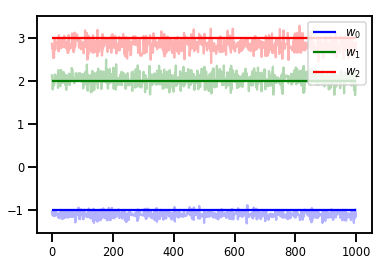
# Trace plots
colors = ['b', 'g', 'r']
for i in range(3):
  plt.plot(samples[:, i], c=colors[i], alpha=.3)
  plt.hlines(true_w[i], 0, 1000, zorder=4, color=colors[i], label="$w_{}$".format(i))
plt.legend(loc='upper right')
plt.show()

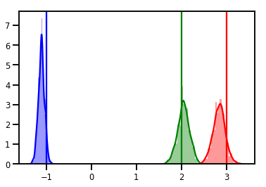
# Histogram of samples
for i in range(3):
  sns.distplot(samples[:, i], color=colors[i])
ymax = plt.ylim()[1]
for i in range(3):
  plt.vlines(true_w[i], 0, ymax, color=colors[i])
plt.ylim(0, ymax)
plt.show()

診断

プロットのトレーシングは悪い方法であありませんが、診断の方が優れています！

まず、複数のチェーンを実行する必要があります。これは、initial_state テンソルのバッチを指定するだけで行えます。

# Instead of a single set of initial w's, we create a batch of 8.
num_chains = 8
initial_state = np.zeros([num_chains, num_features + 1])

chains, kernel_results = run_chain(initial_state)

r_hat = tfp.mcmc.potential_scale_reduction(chains)
print("Acceptance rate:", kernel_results.inner_results.is_accepted.numpy().mean())
print("R-hat diagnostic (per latent variable):", r_hat.numpy())

Acceptance rate: 0.59175
R-hat diagnostic (per latent variable): [0.99998395 0.99932185 0.9997064 ]

ノイズスケールのサンプリング

# Define the joint_log_prob function, and our unnormalized posterior.
def joint_log_prob(w, sigma, x, y):
  # Our model in maths is
  #   w ~ MVN([0, 0, 0], diag([1, 1, 1]))
  #   y_i ~ Normal(w @ x_i, noise_scale),  i=1..N

  rv_w = tfd.MultivariateNormalDiag(
    loc=np.zeros(num_features + 1),
    scale_diag=np.ones(num_features + 1))

  rv_sigma = tfd.LogNormal(np.float64(1.), np.float64(5.))

  rv_y = tfd.Normal(f(x, w), sigma[..., np.newaxis])
  return (rv_w.log_prob(w) +
          rv_sigma.log_prob(sigma) +
          tf.reduce_sum(rv_y.log_prob(y), axis=-1))

# Create our unnormalized target density by currying x and y from the joint.
def unnormalized_posterior(w, sigma):
  return joint_log_prob(w, sigma, xs, ys)


# Create an HMC TransitionKernel
hmc_kernel = tfp.mcmc.HamiltonianMonteCarlo(
  target_log_prob_fn=unnormalized_posterior,
  step_size=np.float64(.1),
  num_leapfrog_steps=4)



# Create a TransformedTransitionKernl
transformed_kernel = tfp.mcmc.TransformedTransitionKernel(
    inner_kernel=hmc_kernel,
    bijector=[tfb.Identity(),    # w
              tfb.Invert(tfb.Softplus())])   # sigma


# Apply a simple step size adaptation during burnin
@tf.function
def run_chain(initial_state, num_results=1000, num_burnin_steps=500):
  adaptive_kernel = tfp.mcmc.SimpleStepSizeAdaptation(
      transformed_kernel,
      num_adaptation_steps=int(.8 * num_burnin_steps),
      target_accept_prob=np.float64(.75))

  return tfp.mcmc.sample_chain(
    num_results=num_results,
    num_burnin_steps=num_burnin_steps,
    current_state=initial_state,
    kernel=adaptive_kernel,
    seed=(0, 1),
    trace_fn=lambda cs, kr: kr)


# Instead of a single set of initial w's, we create a batch of 8.
num_chains = 8
initial_state = [np.zeros([num_chains, num_features + 1]),
                 .54 * np.ones([num_chains], dtype=np.float64)]

chains, kernel_results = run_chain(initial_state)

r_hat = tfp.mcmc.potential_scale_reduction(chains)
print("Acceptance rate:", kernel_results.inner_results.inner_results.is_accepted.numpy().mean())
print("R-hat diagnostic (per w variable):", r_hat[0].numpy())
print("R-hat diagnostic (sigma):", r_hat[1].numpy())

Acceptance rate: 0.715875
R-hat diagnostic (per w variable): [1.0000073  1.00458208 1.00450512]
R-hat diagnostic (sigma): 1.0092056996149859

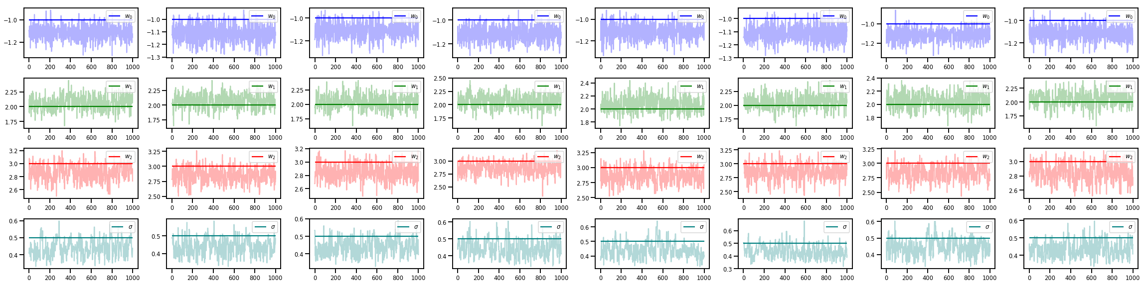
w_chains, sigma_chains = chains

# Trace plots of w (one of 8 chains)
colors = ['b', 'g', 'r', 'teal']
fig, axes = plt.subplots(4, num_chains, figsize=(4 * num_chains, 8))
for j in range(num_chains):
  for i in range(3):
    ax = axes[i][j]
    ax.plot(w_chains[:, j, i], c=colors[i], alpha=.3)
    ax.hlines(true_w[i], 0, 1000, zorder=4, color=colors[i], label="$w_{}$".format(i))
    ax.legend(loc='upper right')
  ax = axes[3][j]
  ax.plot(sigma_chains[:, j], alpha=.3, c=colors[3])
  ax.hlines(noise_scale, 0, 1000, zorder=4, color=colors[3], label=r"$\sigma$".format(i))
  ax.legend(loc='upper right')
fig.tight_layout()
plt.show()

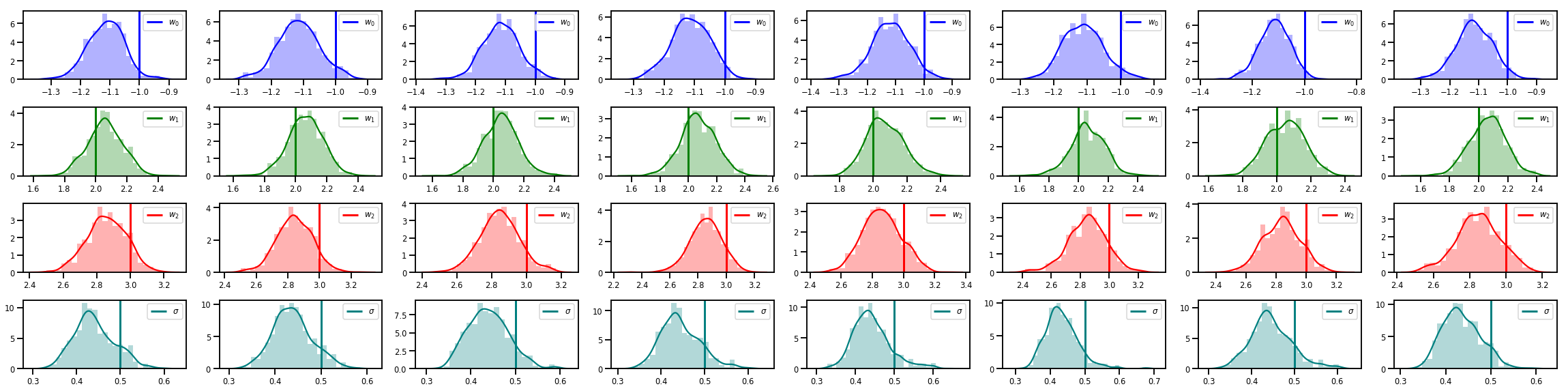
# Histogram of samples of w
fig, axes = plt.subplots(4, num_chains, figsize=(4 * num_chains, 8))
for j in range(num_chains):
  for i in range(3):
    ax = axes[i][j]
    sns.distplot(w_chains[:, j, i], color=colors[i], norm_hist=True, ax=ax, hist_kws={'alpha': .3})
  for i in range(3):
    ax = axes[i][j]
    ymax = ax.get_ylim()[1]
    ax.vlines(true_w[i], 0, ymax, color=colors[i], label="$w_{}$".format(i), linewidth=3)
    ax.set_ylim(0, ymax)
    ax.legend(loc='upper right')


  ax = axes[3][j]
  sns.distplot(sigma_chains[:, j], color=colors[3], norm_hist=True, ax=ax, hist_kws={'alpha': .3})
  ymax = ax.get_ylim()[1]
  ax.vlines(noise_scale, 0, ymax, color=colors[3], label=r"$\sigma$".format(i), linewidth=3)
  ax.set_ylim(0, ymax)
  ax.legend(loc='upper right')
fig.tight_layout()
plt.show()

その他のリソース

次の素晴らしいブログ記事と例をご覧ください。

• 構造時系列のサポート ブログ Colab
• 確率論的 Keras レイヤー（入力: テンソル、出力: 分布！）ブログ Colab
  • レイヤーのもう一つの例: VAE ブログ Colab
• ガウス処理回帰 Colab および潜在変数モデリング Colab

その他の例とノートブックは、こちらの GitHub をご覧ください！