
 GitHub でソースを表示 GitHub でソースを表示 |
Install
TF_Installation = 'System'

if TF_Installation == 'TF Nightly':
  !pip install -q --upgrade tf-nightly
  print('Installation of `tf-nightly` complete.')
elif TF_Installation == 'TF Stable':
  !pip install -q --upgrade tensorflow
  print('Installation of `tensorflow` complete.')
elif TF_Installation == 'System':
  pass
else:
  raise ValueError('Selection Error: Please select a valid '
                   'installation option.')
Install
TFP_Installation = "System"

if TFP_Installation == "Nightly":
  !pip install -q tfp-nightly
  print("Installation of `tfp-nightly` complete.")
elif TFP_Installation == "Stable":
  !pip install -q --upgrade tensorflow-probability
  print("Installation of `tensorflow-probability` complete.")
elif TFP_Installation == "System":
  pass
else:
  raise ValueError("Selection Error: Please select a valid "
                   "installation option.")
概要
このコラボでは、TensorFlow Probability の変分推論を使用して、一般化線形混合効果モデルを適合させる方法を示します。
モデルの族
一般化線形混合効果モデル (GLMM) は、一般化線形モデル (GLM) と似ていますが、予測される線形応答にサンプル固有のノイズが組み込まれている点が異なります。これは、まれな特徴がより一般的に見られる特徴と情報を共有できるため、有用な場合もあります。
生成プロセスとして、一般化線形混合効果モデル (GLMM) には次の特徴があります。
\[ \begin{align} \text{for } & r = 1\ldots R: \hspace{2.45cm}\text{# for each random-effect group}\ &\begin{aligned} \text{for } &c = 1\ldots |C_r|: \hspace{1.3cm}\text{# for each category ("level") of group $r$}\ &\begin{aligned} \beta_{rc} &\sim \text{MultivariateNormal}(\text{loc}=0_{D_r}, \text{scale}=\Sigma_r^{1/2}) \end{aligned} \end{aligned}\\ \text{for } & i = 1 \ldots N: \hspace{2.45cm}\text{# for each sample}\ &\begin{aligned} &\eta_i = \underbrace{\vphantom{\sum_{r=1}^R}x_i^\top\omega}<em data-md-type="emphasis">\text{fixed-effects} + \underbrace{\sum</em>{r=1}^R z_{r,i}^\top \beta_{r,C_r(i) } }<em data-md-type="emphasis">\text{random-effects} \ &Y_i|x_i,\omega,{z</em>{r,i} , \beta_r}_{r=1}^R \sim \text{Distribution}(\text{mean}= g^{-1}(\eta_i)) \end{aligned} \end{align} \]
ここでは、
\[ \begin{align} R &= \text{number of random-effect groups}\ |C_r| &= \text{number of categories for group $r$}\ N &= \text{number of training samples}\ x_i,\omega &\in \mathbb{R}^{D_0}\ D_0 &= \text{number of fixed-effects}\ C_r(i) &= \text{category (under group $r$) of the $i$th sample}\ z_{r,i} &\in \mathbb{R}^{D_r}\ D_r &= \text{number of random-effects associated with group $r$}\ \Sigma_{r} &\in {S\in\mathbb{R}^{D_r \times D_r} : S \succ 0 }\ \eta_i\mapsto g^{-1}(\eta_i) &= \mu_i, \text{inverse link function}\ \text{Distribution} &=\text{some distribution parameterizable solely by its mean} \end{align} \]
つまり、各グループのすべてのカテゴリが、多変量正規分布からのサンプル \(\beta_{rc}\) に関連付けられていることを意味します。\(\beta_{rc}\) の抽出は常に独立していますが、グループ \(r\) に対してのみ同じように分散されます。\(r\in{1,\ldots,R}\) ごとに 1 つの \(\Sigma_r\) があることに注意してください。
サンプルのグループの特徴である \(z_{r,i}\) と密接に組み合わせると、結果は \(i\) 番目の予測線形応答 (それ以外の場合は \(x_i^\top\omega\)) のサンプル固有のノイズになります。
\({\Sigma_r:r\in{1,\ldots,R} }\) を推定する場合、基本的に、変量効果グループがもつノイズの量を推定します。そうしないと、 \(x_i^\top\omega\) に存在する信号が失われます。
\(\text{Distribution}\) および逆リンク関数 \(g^{-1}\) にはさまざまなオプションがあります。一般的なオプションは次のとおりです。
- \(Y_i\sim\text{Normal}(\text{mean}=\eta_i, \text{scale}=\sigma)\),
- \(Y_i\sim\text{Binomial}(\text{mean}=n_i \cdot \text{sigmoid}(\eta_i), \text{total_count}=n_i)\), and,
- \(Y_i\sim\text{Poisson}(\text{mean}=\exp(\eta_i))\).
その他のオプションについては、tfp.glm モジュールを参照してください。
変分推論
残念ながら、パラメータ \(\beta,{\Sigma_r}_r^R\) の最尤推定値を見つけるには、非分析積分が必要です。この問題を回避するためには、
- 付録で \(q_{\lambda}\) と示されている、パラメータ化された分布のファミリ (「代理密度」) を定義します。
- \(q_{\lambda}\) が実際の目標密度に近くなるように、パラメータ \(\lambda\) を見つけます。
分布族は、適切な次元の独立したガウス分布になり、「目標密度に近い」とは、「カルバック・ライブラー情報量を最小化する」ことを意味します。導出と動機については、「変分推論:統計家のためのレビュー」のセクション 2.2 を参照してください。特に、K-L 情報量を最小化することは、負の変分証拠の下限 (ELBO) を最小限に抑えることと同じであることが示されています。
トイプロブレム
Gelman et al. (2007) の「ラドンデータセット」は、回帰のアプローチを示すために使用されるデータセットです。(密接に関連する PyMC3 ブログ記事を参照してください。) ラドンデータセットには、米国全体で取得されたラドンの屋内測定値が含まれています。ラドンは、高濃度で有毒な自然発生の放射性ガスです。
このデモでは、地下室がある家屋ではラドンレベルが高いという仮説を検証することに関心があると仮定します。また、ラドン濃度は土壌の種類、つまり地理的な問題に関連していると考えられます。
これを機械学習の問題としてフレーム化するために、測定が行われた階の線形関数に基づいて対数ラドンレベルを予測します。また、郡を変量効果として使用し、地理的条件による差異を考慮します。つまり、一般化線形混合効果モデルを使用します。
%matplotlib inline
%config InlineBackend.figure_format = 'retina'

import os
from six.moves import urllib

import matplotlib.pyplot as plt; plt.style.use('ggplot')
import numpy as np
import pandas as pd
import seaborn as sns; sns.set_context('notebook')
import tensorflow_datasets as tfds

import tensorflow.compat.v2 as tf
tf.enable_v2_behavior()

import tensorflow_probability as tfp
tfd = tfp.distributions
tfb = tfp.bijectors
また、GPU の可用性を確認します。
if tf.test.gpu_device_name() != '/device:GPU:0':
  print("We'll just use the CPU for this run.")
else:
  print('Huzzah! Found GPU: {}'.format(tf.test.gpu_device_name()))
We'll just use the CPU for this run.
データセットの取得:
TensorFlow データセットからデータセットを読み込み、簡単な前処理を行います。
def load_and_preprocess_radon_dataset(state='MN'):
  """Load the Radon dataset from TensorFlow Datasets and preprocess it.

  Following the examples in "Bayesian Data Analysis" (Gelman, 2007), we filter
  to Minnesota data and preprocess to obtain the following features:
  - `county`: Name of county in which the measurement was taken.
  - `floor`: Floor of house (0 for basement, 1 for first floor) on which the
    measurement was taken.

  The target variable is `log_radon`, the log of the Radon measurement in the
  house.
  """
  ds = tfds.load('radon', split='train')
  radon_data = tfds.as_dataframe(ds)
  radon_data.rename(lambda s: s[9:] if s.startswith('feat') else s, axis=1, inplace=True)
  df = radon_data[radon_data.state==state.encode()].copy()

  df['radon'] = df.activity.apply(lambda x: x if x > 0. else 0.1)
  # Make county names look nice.
  df['county'] = df.county.apply(lambda s: s.decode()).str.strip().str.title()
  # Remap categories to start from 0 and end at max(category).
  df['county'] = df.county.astype(pd.api.types.CategoricalDtype())
  df['county_code'] = df.county.cat.codes
  # Radon levels are all positive, but log levels are unconstrained
  df['log_radon'] = df['radon'].apply(np.log)

  # Drop columns we won't use and tidy the index
  columns_to_keep = ['log_radon', 'floor', 'county', 'county_code']
  df = df[columns_to_keep].reset_index(drop=True)

  return df

df = load_and_preprocess_radon_dataset()
df.head()
GLMM 族の特化
このセクションでは、GLMM 族をラドンレベルの予測タスクに特化します。これを行うには、まず GLMM の固定効果の特殊なケースを検討します: \( \mathbb{E}[\log(\text{radon}_j)] = c + \text{floor_effect}_j \)
このモデルは、観測値 \(j\) の対数ラドンが (予想では) \(j\) 番目の測定が行われる階と一定の切片によって支配されることを前提としています。擬似コードでは、次のようになります。
def estimate_log_radon(floor):
    return intercept + floor_effect[floor]
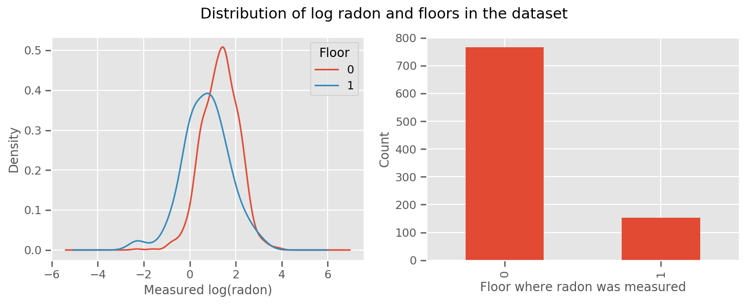
すべての階で学習された重みと、普遍的な intercept の条件があります。0 階と 1 階からのラドン測定値を見ると、これは良いスタートのように見えます。
fig, (ax1, ax2) = plt.subplots(ncols=2, figsize=(12, 4))
df.groupby('floor')['log_radon'].plot(kind='density', ax=ax1);
ax1.set_xlabel('Measured log(radon)')
ax1.legend(title='Floor')

df['floor'].value_counts().plot(kind='bar', ax=ax2)
ax2.set_xlabel('Floor where radon was measured')
ax2.set_ylabel('Count')
fig.suptitle("Distribution of log radon and floors in the dataset");
モデルをもう少し洗練されたものにするために、地理に関することを含めるとさらに良いでしょう。ラドンは土壌に含まれるウランの放射壊変により生ずるため、地理が重要であると考えられます。
擬似コードは次のとおりです。
郡固有の重みを除いて、以前と同じです。
\[ \mathbb{E}[\log(\text{radon}_j)] = c + \text{floor_effect}_j + \text{county_effect}_j \]
郡固有の重みを除いて、以前と同じです。
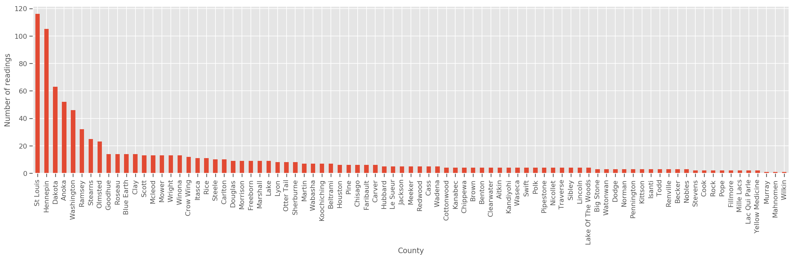
十分に大きなトレーニングセットなので、これは妥当なモデルです。ただし、ミネソタ州からのデータを見てみると、測定数が少ない郡が多数あります。たとえば、85 の郡のうち 39 の郡の観測値は 5 つ未満です。
そのため、郡ごとの観測数が増えるにつれて上記のモデルに収束するように、すべての観測間で統計的強度を共有するようにします。
fig, ax = plt.subplots(figsize=(22, 5));
county_freq = df['county'].value_counts()
county_freq.plot(kind='bar', ax=ax)
ax.set_xlabel('County')
ax.set_ylabel('Number of readings');
このモデルを適合させると、county_effect ベクトルは、トレーニングサンプルが少ない郡の結果を記憶することになり、おそらく過適合になり、一般化が不十分になります。
GLMM は、上記の 2 つの GLM の中間に位置します。以下の適合を検討します。
このモデルは最初のモデルと同じですが、正規分布になる可能性を修正し、(単一の) 変数 county_scale を介してすべての郡で分散を共有します。擬似コードは、以下のとおりです。
観測データを使用して、county_scale、county_mean および random_effect の同時分布を推測します。グローバルな county_scale を使用すると、郡間で統計的強度を共有できます。観測値が多い郡は、観測値が少ない郡の分散を強化します。さらに、より多くのデータを収集すると、このモデルは、プールされたスケール変数のないモデルに収束します。このデータセットを使用しても、どちらのモデルでも最も観察された郡について同様の結論に達します。
\[ \log(\text{radon}_j) \sim c + \text{floor_effect}_j + \mathcal{N}(\text{county_effect}_j, \text{county_scale}) \]
観測データを使用して、county_scale、county_mean および random_effect の同時分布を推測します。グローバルな county_scale を使用すると、郡間で統計的強度を共有できます。観測値が多い郡は、観測値が少ない郡の分散を強化します。さらに、より多くのデータを収集すると、このモデルは、プールされたスケール変数のないモデルに収束します。このデータセットを使用しても、どちらのモデルでも最も観察された郡について同様の結論に達します。
実験
次に、TensorFlow の変分推論を使用して、上記の GLMM を適合させます。まず、データを特徴とラベルに分割します。
features = df[['county_code', 'floor']].astype(int)
labels = df[['log_radon']].astype(np.float32).values.flatten()
モデルの指定
def make_joint_distribution_coroutine(floor, county, n_counties, n_floors):

  def model():
    county_scale = yield tfd.HalfNormal(scale=1., name='scale_prior')
    intercept = yield tfd.Normal(loc=0., scale=1., name='intercept')
    floor_weight = yield tfd.Normal(loc=0., scale=1., name='floor_weight')
    county_prior = yield tfd.Normal(loc=tf.zeros(n_counties),
                                    scale=county_scale,
                                    name='county_prior')
    random_effect = tf.gather(county_prior, county, axis=-1)

    fixed_effect = intercept + floor_weight * floor
    linear_response = fixed_effect + random_effect
    yield tfd.Normal(loc=linear_response, scale=1., name='likelihood')
  return tfd.JointDistributionCoroutineAutoBatched(model)

joint = make_joint_distribution_coroutine(
    features.floor.values, features.county_code.values, df.county.nunique(),
    df.floor.nunique())

# Define a closure over the joint distribution
# to condition on the observed labels.
def target_log_prob_fn(*args):
  return joint.log_prob(*args, likelihood=labels)
事後分布を指定する
ここで、サロゲート族 \(q_{\lambda}\) を作成しました。パラメータ \(\lambda\) はトレーニング可能です。この場合、分布族は、パラメータごとに 1 つずつ、独立した多変量正規分布であり、\(\lambda = {(\mu_j, \sigma_j)}\) です。\(j\) は 4 つのパラメータにインデックスを付けます。
サロゲート分布族を適合させるために使用するメソッドは、tf.Variables を使用します。また、tfp.util.TransformedVariable を Softplus とともに使用して、(トレーニング可能な) スケールパラメータを正に制約します。また、tfp.util.TransformedVariableを Softplus とともに使用して、(トレーニング可能な) スケールパラメータを正に制約します。
最適化を支援するために、これらのトレーニング可能な変数を初期化します。
# Initialize locations and scales randomly with `tf.Variable`s and
# `tfp.util.TransformedVariable`s.
_init_loc = lambda shape=(): tf.Variable(
    tf.random.uniform(shape, minval=-2., maxval=2.))
_init_scale = lambda shape=(): tfp.util.TransformedVariable(
    initial_value=tf.random.uniform(shape, minval=0.01, maxval=1.),
    bijector=tfb.Softplus())
n_counties = df.county.nunique()

surrogate_posterior = tfd.JointDistributionSequentialAutoBatched([
  tfb.Softplus()(tfd.Normal(_init_loc(), _init_scale())),           # scale_prior
  tfd.Normal(_init_loc(), _init_scale()),                           # intercept
  tfd.Normal(_init_loc(), _init_scale()),                           # floor_weight
  tfd.Normal(_init_loc([n_counties]), _init_scale([n_counties]))])  # county_prior
このセルは、次のように tfp.experimental.vi.build_factored_surrogate_posterior に置き換えることができることに注意してください。
surrogate_posterior = tfp.experimental.vi.build_factored_surrogate_posterior(
  event_shape=joint.event_shape_tensor()[:-1],
  constraining_bijectors=[tfb.Softplus(), None, None, None])
結果
ここでの目標は、扱いやすいパラメータ化された分布族を定義し、パラメータを選択して、ターゲット分布に近い扱いやすい分布を作成することでした。
上記のようにサロゲート分布を作成し、 tfp.vi.fit_surrogate_posterior を使用できます。これは、オプティマイザと指定された数のステップを受け入れて、負の ELBO を最小化するサロゲートモデルのパラメータを見つけます (これは、サロゲート分布とターゲット分布の間のカルバック・ライブラー情報を最小化することに対応します)。
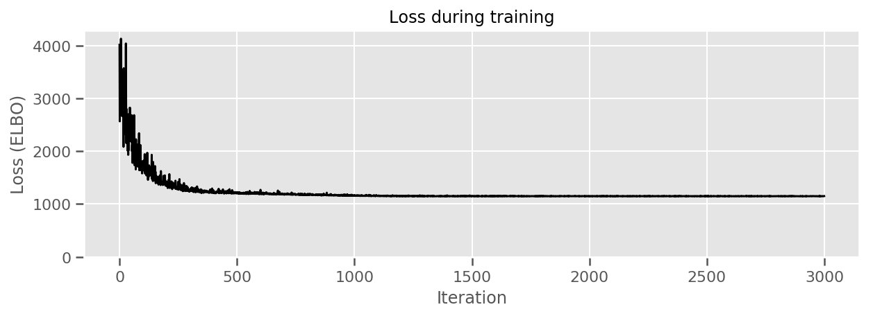
戻り値は各ステップで負の ELBO であり、surrogate_posterior の分布はオプティマイザによって検出されたパラメータで更新されます。
optimizer = tf.optimizers.Adam(learning_rate=1e-2)

losses = tfp.vi.fit_surrogate_posterior(
    target_log_prob_fn,
    surrogate_posterior,
    optimizer=optimizer,
    num_steps=3000,
    seed=42,
    sample_size=2)

(scale_prior_,
 intercept_,
 floor_weight_,
 county_weights_), _ = surrogate_posterior.sample_distributions()
print('        intercept (mean): ', intercept_.mean())
print('     floor_weight (mean): ', floor_weight_.mean())
print(' scale_prior (approx. mean): ', tf.reduce_mean(scale_prior_.sample(10000)))
intercept (mean):  tf.Tensor(1.4352839, shape=(), dtype=float32)
     floor_weight (mean):  tf.Tensor(-0.6701997, shape=(), dtype=float32)
 scale_prior (approx. mean):  tf.Tensor(0.28682157, shape=(), dtype=float32)
fig, ax = plt.subplots(figsize=(10, 3))
ax.plot(losses, 'k-')
ax.set(xlabel="Iteration",
       ylabel="Loss (ELBO)",
       title="Loss during training",
       ylim=0);
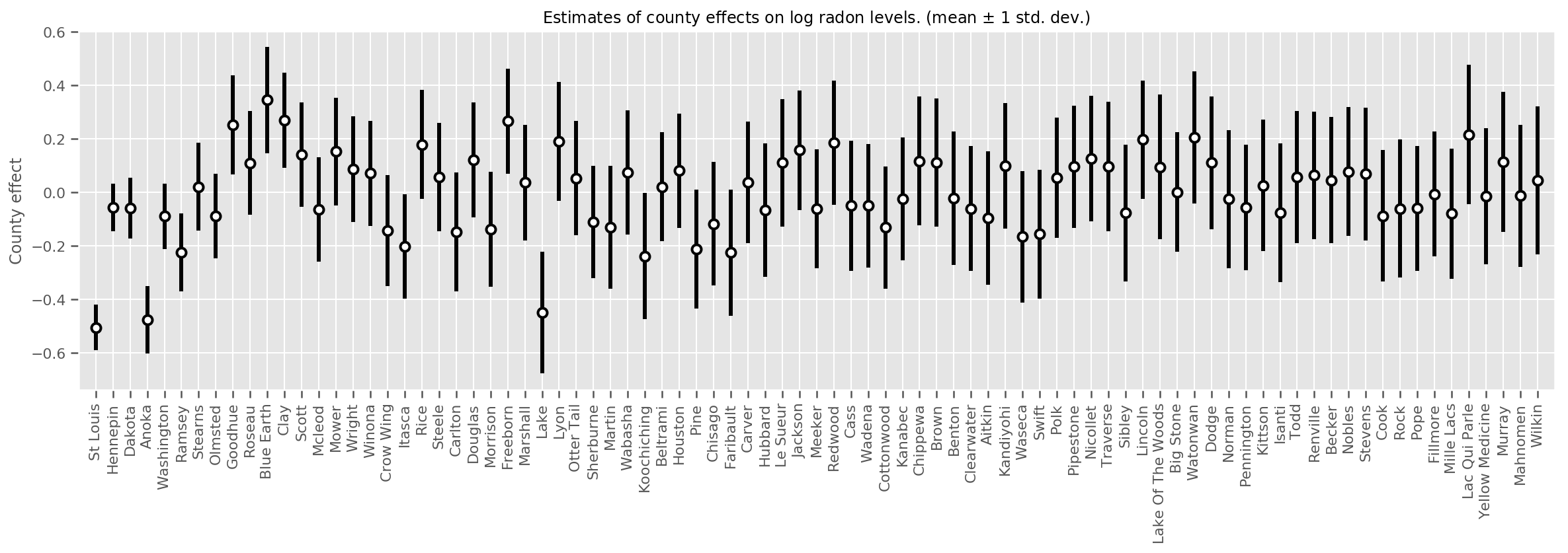
推定された平均郡効果をその平均の不確実性とともにプロットし、観測数で並べ替えました。左側が最大です。観測値が多い郡では不確実性は小さく、観測値が 1 つか 2 つしかない郡では不確実性が大きいことに注意してください。
county_counts = (df.groupby(by=['county', 'county_code'], observed=True)
                   .agg('size')
                   .sort_values(ascending=False)
                   .reset_index(name='count'))

means = county_weights_.mean()
stds = county_weights_.stddev()

fig, ax = plt.subplots(figsize=(20, 5))

for idx, row in county_counts.iterrows():
  mid = means[row.county_code]
  std = stds[row.county_code]
  ax.vlines(idx, mid - std, mid + std, linewidth=3)
  ax.plot(idx, means[row.county_code], 'ko', mfc='w', mew=2, ms=7)

ax.set(
    xticks=np.arange(len(county_counts)),
    xlim=(-1, len(county_counts)),
    ylabel="County effect",
    title=r"Estimates of county effects on log radon levels. (mean $\pm$ 1 std. dev.)",
)
ax.set_xticklabels(county_counts.county, rotation=90);
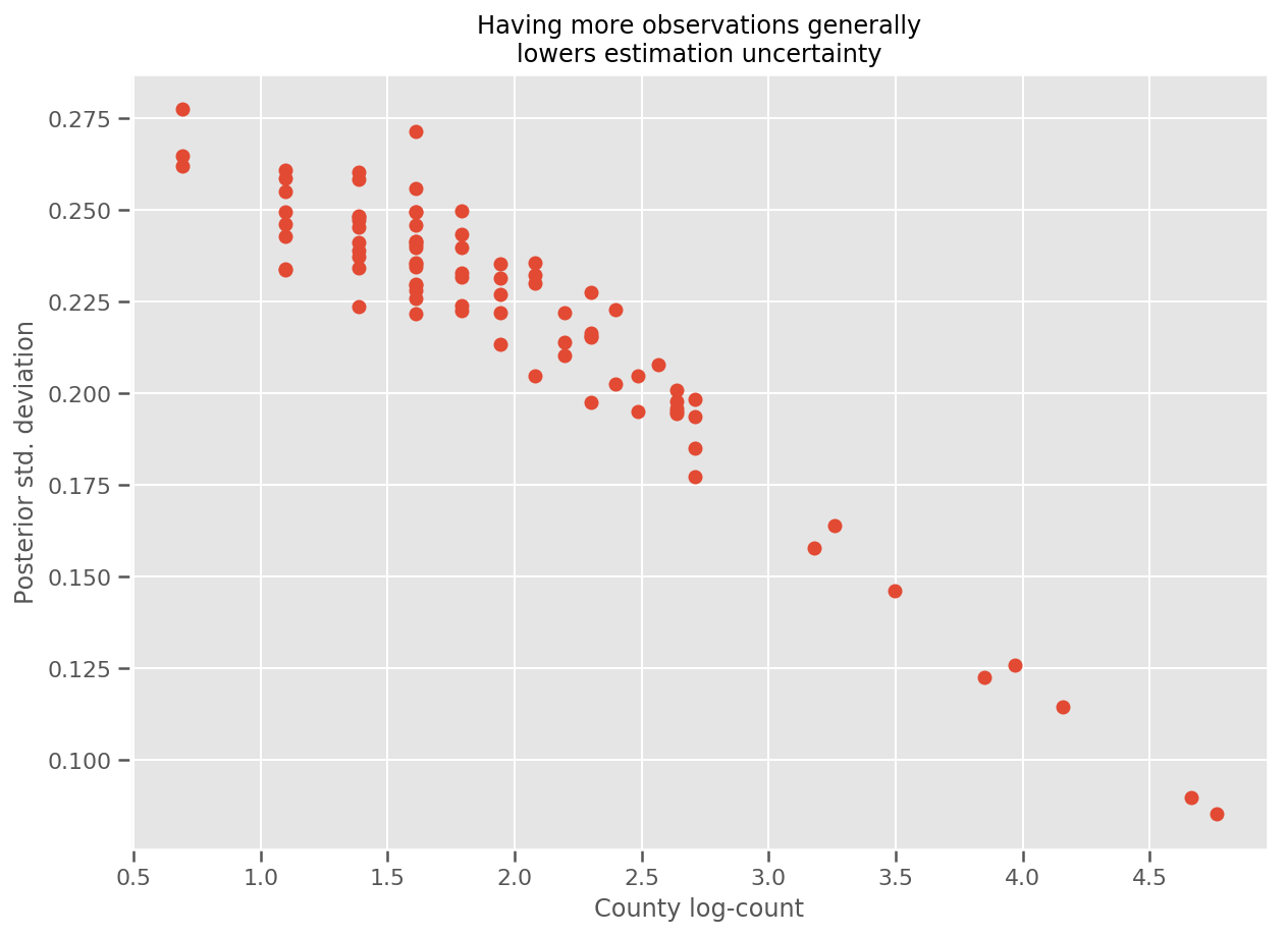
実際、推定された標準偏差に対して観測値の対数をプロットすることで、このことを直接に確認でき、関係がほぼ線形であることがわかります。
fig, ax = plt.subplots(figsize=(10, 7))
ax.plot(np.log1p(county_counts['count']), stds.numpy()[county_counts.county_code], 'o')
ax.set(
    ylabel='Posterior std. deviation',
    xlabel='County log-count',
    title='Having more observations generally\nlowers estimation uncertainty'
);
R の lme4 との比較
%%shell
exit  # Trick to make this block not execute.

radon = read.csv('srrs2.dat', header = TRUE)
radon = radon[radon$state=='MN',]
radon$radon = ifelse(radon$activity==0., 0.1, radon$activity)
radon$log_radon = log(radon$radon)

# install.packages('lme4')
library(lme4)
fit <- lmer(log_radon ~ 1 + floor + (1 | county), data=radon)
fit

# Linear mixed model fit by REML ['lmerMod']
# Formula: log_radon ~ 1 + floor + (1 | county)
#    Data: radon
# REML criterion at convergence: 2171.305
# Random effects:
#  Groups   Name        Std.Dev.
#  county   (Intercept) 0.3282
#  Residual             0.7556
# Number of obs: 919, groups:  county, 85
# Fixed Effects:
# (Intercept)        floor
#       1.462       -0.693
<IPython.core.display.Javascript at 0x7f90b888e9b0>
<IPython.core.display.Javascript at 0x7f90b888e780>
<IPython.core.display.Javascript at 0x7f90b888e780>
<IPython.core.display.Javascript at 0x7f90bce1dfd0>
<IPython.core.display.Javascript at 0x7f90b888e780>
<IPython.core.display.Javascript at 0x7f90b888e780>
<IPython.core.display.Javascript at 0x7f90b888e780>
<IPython.core.display.Javascript at 0x7f90b888e780>
次の表は、結果をまとめたものです。
print(pd.DataFrame(data=dict(intercept=[1.462, tf.reduce_mean(intercept_.mean()).numpy()],
                             floor=[-0.693, tf.reduce_mean(floor_weight_.mean()).numpy()],
                             scale=[0.3282, tf.reduce_mean(scale_prior_.sample(10000)).numpy()]),
                   index=['lme4', 'vi']))
intercept   floor     scale
lme4   1.462000 -0.6930  0.328200
vi     1.435284 -0.6702  0.287251
この表は、VI の結果が lme4 の約 10% 以内であることを示しています。これは、次の理由からやや驚くべきことです。
lme4はラプラスの方法 (VI ではない) に基づく- このコラボでは、実際に収束するように努力していない
- ハイパーパラメータを調整するための労力は最小限
- データを正規化または前処理するために努力していない (中心の特徴などは考慮されていない)。
結論
このコラボでは、一般化線形混合効果モデルについて説明し、TensorFlow Probability を使用して変分推論を使用してそれらを適合させる方法を示しました。トイプロブレムには数百のトレーニングサンプルしかありませんでしたが、ここで使用した手法は、大規模な場合でも使用できます。