このノートブックでは、構造時系列モデルを時系列に適合する例とそれを使用して予測と説明を生成する例を説明しています。
| |
 GitHub でソースを表示 GitHub でソースを表示 |
依存関係と前提条件
Import and set ups
%matplotlib inline
import matplotlib as mpl
from matplotlib import pylab as plt
import matplotlib.dates as mdates
import seaborn as sns

import collections

import numpy as np
import tensorflow.compat.v2 as tf
import tensorflow_probability as tfp

from tensorflow_probability import distributions as tfd
from tensorflow_probability import sts

tf.enable_v2_behavior()
迅速に作成
はじめる前に、このデモに GPU を使用していることを確認します。
これを行うには、[ランタイム]->[ランタイムタイプの変更]->[ハードウェアアクセラレータ]->[GPU]を選択します。
次のスニペットは、GPU にアクセスできることを確認します。
if tf.test.gpu_device_name() != '/device:GPU:0':
  print('WARNING: GPU device not found.')
else:
  print('SUCCESS: Found GPU: {}'.format(tf.test.gpu_device_name()))
SUCCESS: Found GPU: /device:GPU:0
注意: 何らかの理由で GPU にアクセスできない場合でも、このコラボは機能します (トレーニングには時間がかかります)。
プロットのセットアップ
時系列と予測をプロットするヘルパーメソッドです。
from pandas.plotting import register_matplotlib_converters
register_matplotlib_converters()

sns.set_context("notebook", font_scale=1.)
sns.set_style("whitegrid")
%config InlineBackend.figure_format = 'retina'
def plot_forecast(x, y,
                  forecast_mean, forecast_scale, forecast_samples,
                  title, x_locator=None, x_formatter=None):
  """Plot a forecast distribution against the 'true' time series."""
  colors = sns.color_palette()
  c1, c2 = colors[0], colors[1]
  fig = plt.figure(figsize=(12, 6))
  ax = fig.add_subplot(1, 1, 1)

  num_steps = len(y)
  num_steps_forecast = forecast_mean.shape[-1]
  num_steps_train = num_steps - num_steps_forecast


  ax.plot(x, y, lw=2, color=c1, label='ground truth')

  forecast_steps = np.arange(
      x[num_steps_train],
      x[num_steps_train]+num_steps_forecast,
      dtype=x.dtype)

  ax.plot(forecast_steps, forecast_samples.T, lw=1, color=c2, alpha=0.1)

  ax.plot(forecast_steps, forecast_mean, lw=2, ls='--', color=c2,
           label='forecast')
  ax.fill_between(forecast_steps,
                   forecast_mean-2*forecast_scale,
                   forecast_mean+2*forecast_scale, color=c2, alpha=0.2)

  ymin, ymax = min(np.min(forecast_samples), np.min(y)), max(np.max(forecast_samples), np.max(y))
  yrange = ymax-ymin
  ax.set_ylim([ymin - yrange*0.1, ymax + yrange*0.1])
  ax.set_title("{}".format(title))
  ax.legend()

  if x_locator is not None:
    ax.xaxis.set_major_locator(x_locator)
    ax.xaxis.set_major_formatter(x_formatter)
    fig.autofmt_xdate()

  return fig, ax
def plot_components(dates,
                    component_means_dict,
                    component_stddevs_dict,
                    x_locator=None,
                    x_formatter=None):
  """Plot the contributions of posterior components in a single figure."""
  colors = sns.color_palette()
  c1, c2 = colors[0], colors[1]

  axes_dict = collections.OrderedDict()
  num_components = len(component_means_dict)
  fig = plt.figure(figsize=(12, 2.5 * num_components))
  for i, component_name in enumerate(component_means_dict.keys()):
    component_mean = component_means_dict[component_name]
    component_stddev = component_stddevs_dict[component_name]

    ax = fig.add_subplot(num_components,1,1+i)
    ax.plot(dates, component_mean, lw=2)
    ax.fill_between(dates,
                     component_mean-2*component_stddev,
                     component_mean+2*component_stddev,
                     color=c2, alpha=0.5)
    ax.set_title(component_name)
    if x_locator is not None:
      ax.xaxis.set_major_locator(x_locator)
      ax.xaxis.set_major_formatter(x_formatter)
    axes_dict[component_name] = ax
  fig.autofmt_xdate()
  fig.tight_layout()
  return fig, axes_dict
def plot_one_step_predictive(dates, observed_time_series,
                             one_step_mean, one_step_scale,
                             x_locator=None, x_formatter=None):
  """Plot a time series against a model's one-step predictions."""

  colors = sns.color_palette()
  c1, c2 = colors[0], colors[1]

  fig=plt.figure(figsize=(12, 6))
  ax = fig.add_subplot(1,1,1)
  num_timesteps = one_step_mean.shape[-1]
  ax.plot(dates, observed_time_series, label="observed time series", color=c1)
  ax.plot(dates, one_step_mean, label="one-step prediction", color=c2)
  ax.fill_between(dates,
                  one_step_mean - one_step_scale,
                  one_step_mean + one_step_scale,
                  alpha=0.1, color=c2)
  ax.legend()

  if x_locator is not None:
    ax.xaxis.set_major_locator(x_locator)
    ax.xaxis.set_major_formatter(x_formatter)
    fig.autofmt_xdate()
  fig.tight_layout()
  return fig, ax
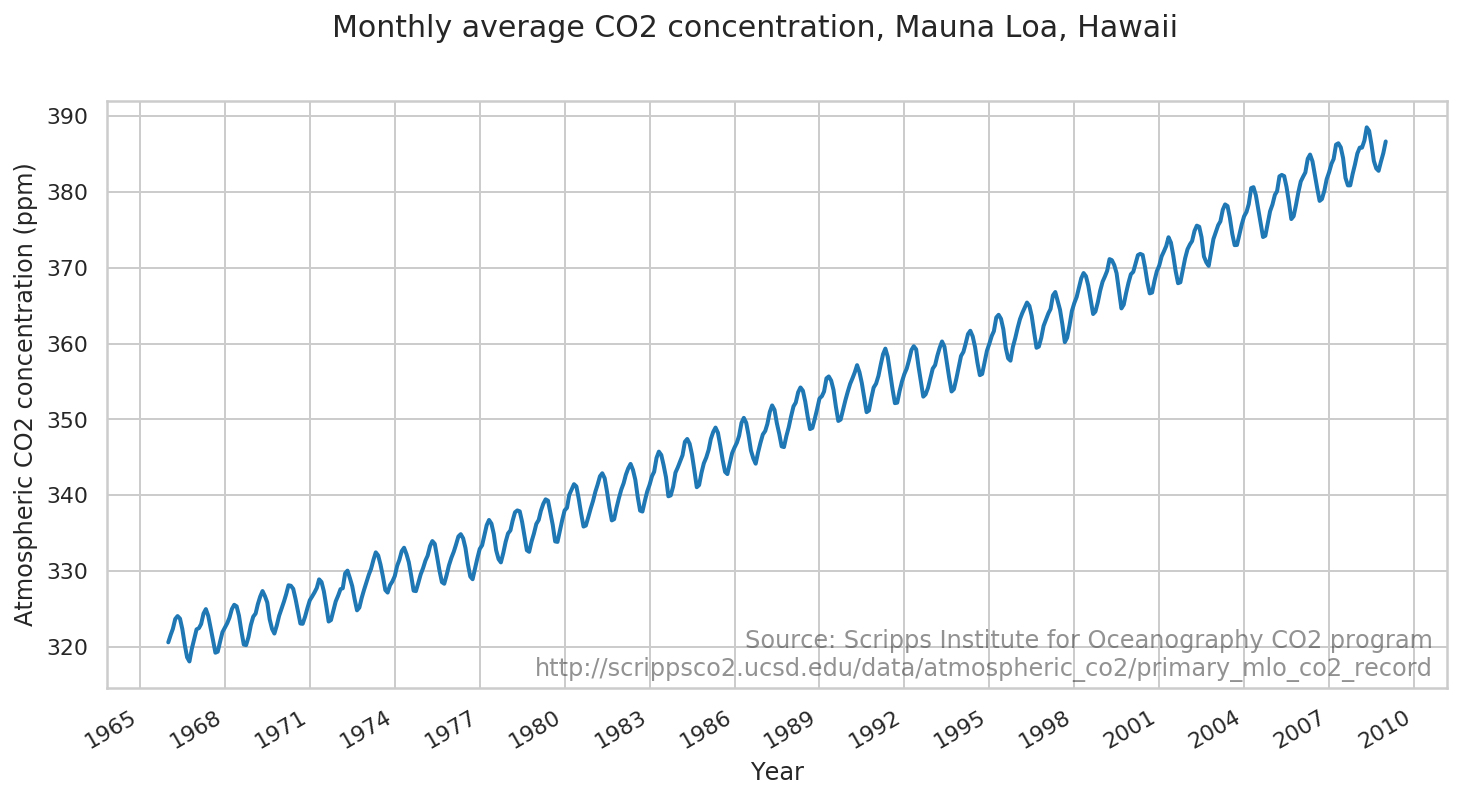
マヌアロアの CO2 の記録
モデルを、マヌアロア観測所から得た大気中の CO2 の読み取りに適合させます。
データ
# CO2 readings from Mauna Loa observatory, monthly beginning January 1966
# Original source: http://scrippsco2.ucsd.edu/data/atmospheric_co2/primary_mlo_co2_record
co2_by_month = np.array('320.62,321.60,322.39,323.70,324.08,323.75,322.38,320.36,318.64,318.10,319.78,321.03,322.33,322.50,323.04,324.42,325.00,324.09,322.54,320.92,319.25,319.39,320.73,321.96,322.57,323.15,323.89,325.02,325.57,325.36,324.14,322.11,320.33,320.25,321.32,322.89,324.00,324.42,325.63,326.66,327.38,326.71,325.88,323.66,322.38,321.78,322.85,324.12,325.06,325.98,326.93,328.14,328.08,327.67,326.34,324.69,323.10,323.06,324.01,325.13,326.17,326.68,327.17,327.79,328.92,328.57,327.36,325.43,323.36,323.56,324.80,326.01,326.77,327.63,327.75,329.73,330.07,329.09,328.04,326.32,324.84,325.20,326.50,327.55,328.55,329.56,330.30,331.50,332.48,332.07,330.87,329.31,327.51,327.18,328.16,328.64,329.35,330.71,331.48,332.65,333.09,332.25,331.18,329.39,327.43,327.37,328.46,329.57,330.40,331.40,332.04,333.31,333.97,333.60,331.90,330.06,328.56,328.34,329.49,330.76,331.75,332.56,333.50,334.58,334.88,334.33,333.05,330.94,329.30,328.94,330.31,331.68,332.93,333.42,334.70,336.07,336.75,336.27,334.92,332.75,331.59,331.16,332.40,333.85,334.97,335.38,336.64,337.76,338.01,337.89,336.54,334.68,332.76,332.55,333.92,334.95,336.23,336.76,337.96,338.88,339.47,339.29,337.73,336.09,333.92,333.86,335.29,336.73,338.01,338.36,340.07,340.77,341.47,341.17,339.56,337.60,335.88,336.02,337.10,338.21,339.24,340.48,341.38,342.51,342.91,342.25,340.49,338.43,336.69,336.86,338.36,339.61,340.75,341.61,342.70,343.57,344.14,343.35,342.06,339.81,337.98,337.86,339.26,340.49,341.38,342.52,343.10,344.94,345.76,345.32,343.98,342.38,339.87,339.99,341.15,342.99,343.70,344.50,345.28,347.06,347.43,346.80,345.39,343.28,341.07,341.35,342.98,344.22,344.97,345.99,347.42,348.35,348.93,348.25,346.56,344.67,343.09,342.80,344.24,345.56,346.30,346.95,347.85,349.55,350.21,349.55,347.94,345.90,344.85,344.17,345.66,346.90,348.02,348.48,349.42,350.99,351.85,351.26,349.51,348.10,346.45,346.36,347.81,348.96,350.43,351.73,352.22,353.59,354.22,353.79,352.38,350.43,348.73,348.88,350.07,351.34,352.76,353.07,353.68,355.42,355.67,355.12,353.90,351.67,349.80,349.99,351.30,352.52,353.66,354.70,355.38,356.20,357.16,356.23,354.81,352.91,350.96,351.18,352.83,354.21,354.72,355.75,357.16,358.60,359.34,358.24,356.17,354.02,352.15,352.21,353.75,354.99,355.99,356.72,357.81,359.15,359.66,359.25,357.02,355.00,353.01,353.31,354.16,355.40,356.70,357.17,358.38,359.46,360.28,359.60,357.57,355.52,353.69,353.99,355.34,356.80,358.37,358.91,359.97,361.26,361.69,360.94,359.55,357.48,355.84,356.00,357.58,359.04,359.97,361.00,361.64,363.45,363.80,363.26,361.89,359.45,358.05,357.75,359.56,360.70,362.05,363.24,364.02,364.71,365.41,364.97,363.65,361.48,359.45,359.61,360.76,362.33,363.18,363.99,364.56,366.36,366.80,365.63,364.47,362.50,360.19,360.78,362.43,364.28,365.33,366.15,367.31,368.61,369.30,368.88,367.64,365.78,363.90,364.23,365.46,366.97,368.15,368.87,369.59,371.14,371.00,370.35,369.27,366.93,364.64,365.13,366.68,368.00,369.14,369.46,370.51,371.66,371.83,371.69,370.12,368.12,366.62,366.73,368.29,369.53,370.28,371.50,372.12,372.86,374.02,373.31,371.62,369.55,367.96,368.09,369.68,371.24,372.44,373.08,373.52,374.85,375.55,375.40,374.02,371.48,370.70,370.25,372.08,373.78,374.68,375.62,376.11,377.65,378.35,378.13,376.61,374.48,372.98,373.00,374.35,375.69,376.79,377.36,378.39,380.50,380.62,379.55,377.76,375.83,374.05,374.22,375.84,377.44,378.34,379.61,380.08,382.05,382.24,382.08,380.67,378.67,376.42,376.80,378.31,379.96,381.37,382.02,382.56,384.37,384.92,384.03,382.28,380.48,378.81,379.06,380.14,381.66,382.58,383.71,384.34,386.23,386.41,385.87,384.45,381.84,380.86,380.86,382.36,383.61,385.07,385.84,385.83,386.77,388.51,388.05,386.25,384.08,383.09,382.78,384.01,385.11,386.65,387.12,388.52,389.57,390.16,389.62,388.07,386.08,384.65,384.33,386.05,387.49,388.55,390.07,391.01,392.38,393.22,392.24,390.33,388.52,386.84,387.16,388.67,389.81,391.30,391.92,392.45,393.37,394.28,393.69,392.59,390.21,389.00,388.93,390.24,391.80,393.07,393.35,394.36,396.43,396.87,395.88,394.52,392.54,391.13,391.01,392.95,394.34,395.61,396.85,397.26,398.35,399.98,398.87,397.37,395.41,393.39,393.70,395.19,396.82,397.92,398.10,399.47,401.33,401.88,401.31,399.07,397.21,395.40,395.65,397.23,398.79,399.85,400.31,401.51,403.45,404.10,402.88,401.61,399.00,397.50,398.28,400.24,401.89,402.65,404.16,404.85,407.57,407.66,407.00,404.50,402.24,401.01,401.50,403.64,404.55,406.07,406.64,407.06,408.95,409.91,409.12,407.20,405.24,403.27,403.64,405.17,406.75,408.05,408.34,409.25,410.30,411.30,410.88,408.90,407.10,405.59,405.99,408.12,409.23,410.92'.split(',')).astype(np.float32)

co2_by_month = co2_by_month
num_forecast_steps = 12 * 10 # Forecast the final ten years, given previous data
co2_by_month_training_data = co2_by_month[:-num_forecast_steps]

co2_dates = np.arange("1966-01", "2019-02", dtype="datetime64[M]")
co2_loc = mdates.YearLocator(3)
co2_fmt = mdates.DateFormatter('%Y')
fig = plt.figure(figsize=(12, 6))
ax = fig.add_subplot(1, 1, 1)
ax.plot(co2_dates[:-num_forecast_steps], co2_by_month_training_data, lw=2, label="training data")
ax.xaxis.set_major_locator(co2_loc)
ax.xaxis.set_major_formatter(co2_fmt)
ax.set_ylabel("Atmospheric CO2 concentration (ppm)")
ax.set_xlabel("Year")
fig.suptitle("Monthly average CO2 concentration, Mauna Loa, Hawaii",
             fontsize=15)
ax.text(0.99, .02,
        "Source: Scripps Institute for Oceanography CO2 program\nhttp://scrippsco2.ucsd.edu/data/atmospheric_co2/primary_mlo_co2_record",
        transform=ax.transAxes,
        horizontalalignment="right",
        alpha=0.5)
fig.autofmt_xdate()
モデルと適合
現地の線形トレンドと月の季節効果を使って、この時系列をモデリングします。
def build_model(observed_time_series):
  trend = sts.LocalLinearTrend(observed_time_series=observed_time_series)
  seasonal = tfp.sts.Seasonal(
      num_seasons=12, observed_time_series=observed_time_series)
  model = sts.Sum([trend, seasonal], observed_time_series=observed_time_series)
  return model
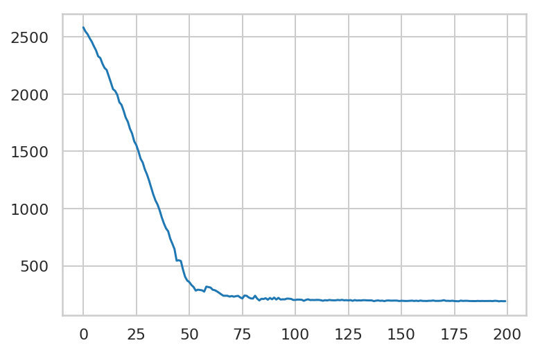
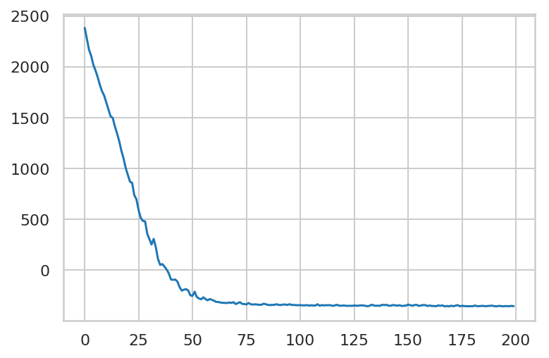
このモデルを、変分推論を使って適合します。これには、変分損失関数の負の証拠下限(ELBO)を最小化するオプティマイザの実行が伴います。これは、パラメータのおおよその事後分布のセットを適合します(実際には、各パラメータの台空間に変換された独立した正規分布であると仮定しています)。
tfp.sts 予測方法には、入力として事後サンプルが必要であるため、変分事後分布から一連のサンプルを描いて終了します。
co2_model = build_model(co2_by_month_training_data)

# Build the variational surrogate posteriors `qs`.
variational_posteriors = tfp.sts.build_factored_surrogate_posterior(
    model=co2_model)
Minimize the variational loss.
# Allow external control of optimization to reduce test runtimes.
num_variational_steps = 200 # @param { isTemplate: true}
num_variational_steps = int(num_variational_steps)

# Build and optimize the variational loss function.
elbo_loss_curve = tfp.vi.fit_surrogate_posterior(
    target_log_prob_fn=co2_model.joint_distribution(
        observed_time_series=co2_by_month_training_data).log_prob,
    surrogate_posterior=variational_posteriors,
    optimizer=tf.optimizers.Adam(learning_rate=0.1),
    num_steps=num_variational_steps,
    jit_compile=True)

plt.plot(elbo_loss_curve)
plt.show()

# Draw samples from the variational posterior.
q_samples_co2_ = variational_posteriors.sample(50)
WARNING:tensorflow:From /usr/local/lib/python3.6/dist-packages/tensorflow_core/python/ops/linalg/linear_operator_diag.py:166: calling LinearOperator.__init__ (from tensorflow.python.ops.linalg.linear_operator) with graph_parents is deprecated and will be removed in a future version.
Instructions for updating:
Do not pass `graph_parents`.  They will  no longer be used.
print("Inferred parameters:")
for param in co2_model.parameters:
  print("{}: {} +- {}".format(param.name,
                              np.mean(q_samples_co2_[param.name], axis=0),
                              np.std(q_samples_co2_[param.name], axis=0)))
Inferred parameters:
observation_noise_scale: 0.17199112474918365 +- 0.009443143382668495
LocalLinearTrend/_level_scale: 0.17671072483062744 +- 0.01510554924607277
LocalLinearTrend/_slope_scale: 0.004302256740629673 +- 0.0018349259626120329
Seasonal/_drift_scale: 0.041069451719522476 +- 0.007772190496325493
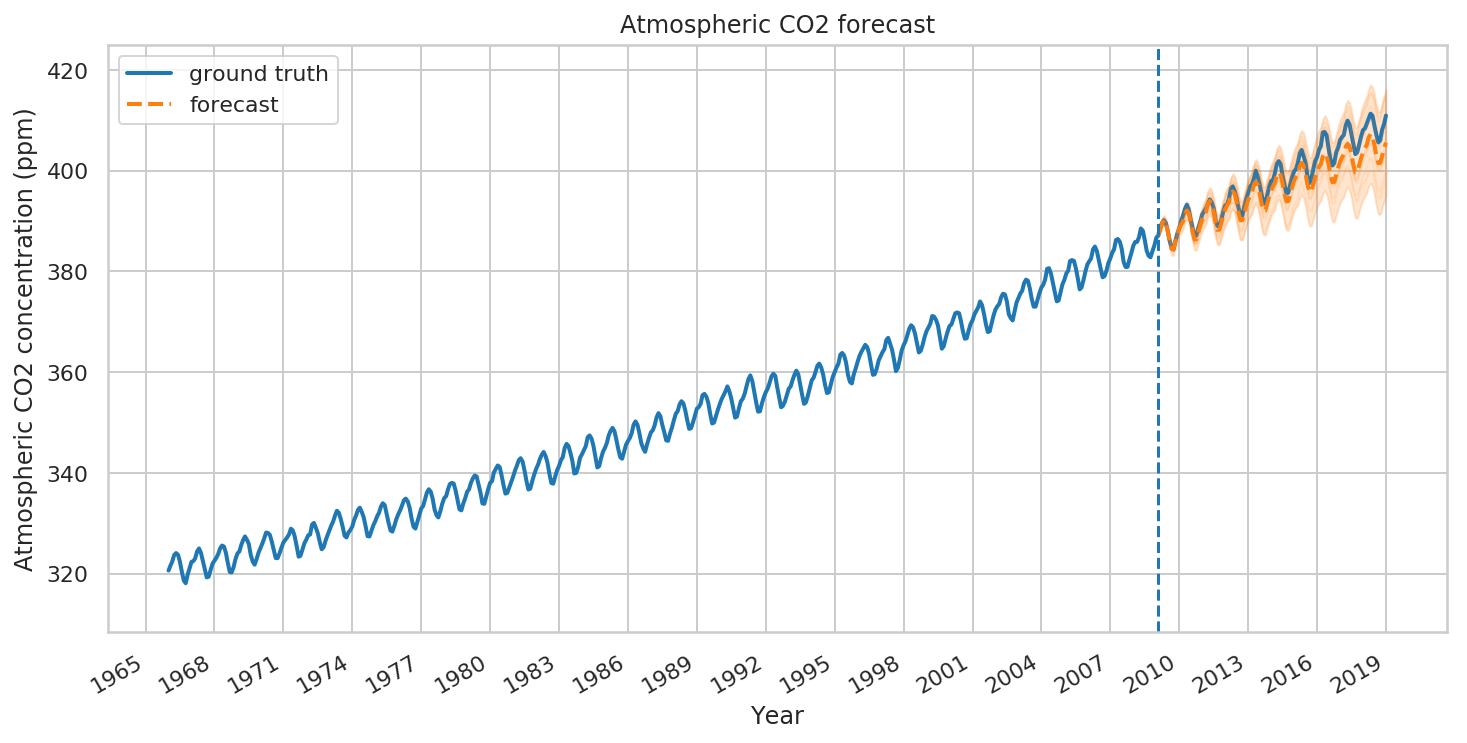
予測と批判
では、適合モデルを使用して、予測を構築しましょう。tfp.sts.forecast を呼び出すだけですが、未来のタイムスタンプで予測分布を表す TensorFlow Distribution インスタンスが返されます。
co2_forecast_dist = tfp.sts.forecast(
    co2_model,
    observed_time_series=co2_by_month_training_data,
    parameter_samples=q_samples_co2_,
    num_steps_forecast=num_forecast_steps)
特に、予測分布の mean と stddev は、各時間ステップでわずかに不確実性を伴う予測を提供するため、可能な未来のサンプルを抽出することもできます。
num_samples=10

co2_forecast_mean, co2_forecast_scale, co2_forecast_samples = (
    co2_forecast_dist.mean().numpy()[..., 0],
    co2_forecast_dist.stddev().numpy()[..., 0],
    co2_forecast_dist.sample(num_samples).numpy()[..., 0])
fig, ax = plot_forecast(
    co2_dates, co2_by_month,
    co2_forecast_mean, co2_forecast_scale, co2_forecast_samples,
    x_locator=co2_loc,
    x_formatter=co2_fmt,
    title="Atmospheric CO2 forecast")
ax.axvline(co2_dates[-num_forecast_steps], linestyle="--")
ax.legend(loc="upper left")
ax.set_ylabel("Atmospheric CO2 concentration (ppm)")
ax.set_xlabel("Year")
fig.autofmt_xdate()
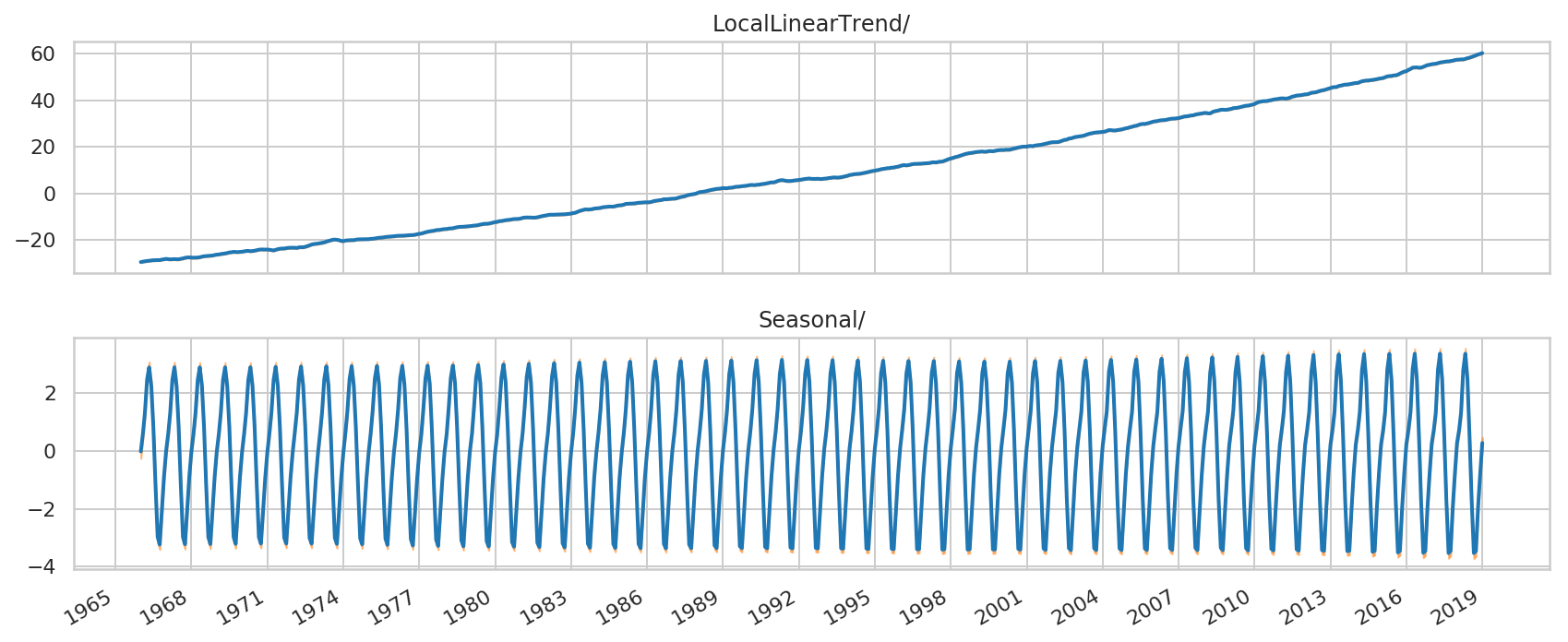
モデルを個々の時系列の貢献に分解することで、モデルの適合性をさらに理解できます。
# Build a dict mapping components to distributions over
# their contribution to the observed signal.
component_dists = sts.decompose_by_component(
    co2_model,
    observed_time_series=co2_by_month,
    parameter_samples=q_samples_co2_)
co2_component_means_, co2_component_stddevs_ = (
    {k.name: c.mean() for k, c in component_dists.items()},
    {k.name: c.stddev() for k, c in component_dists.items()})
_ = plot_components(co2_dates, co2_component_means_, co2_component_stddevs_,
                    x_locator=co2_loc, x_formatter=co2_fmt)
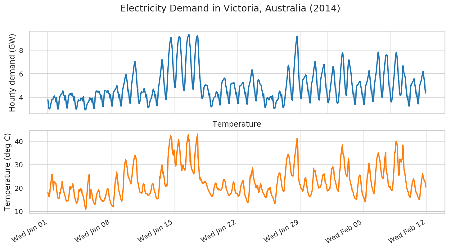
電力の需要の予測
次に、より複雑な例を検討しましょう。オーストラリアのビクトリア州における電力需要の予測です。
まず、データセットを構築します。
# Victoria electricity demand dataset, as presented at
# https://otexts.com/fpp2/scatterplots.html
# and downloaded from https://github.com/robjhyndman/fpp2-package/blob/master/data/elecdaily.rda
# This series contains the first eight weeks (starting Jan 1). The original
# dataset was half-hourly data; here we've downsampled to hourly data by taking
# every other timestep.
demand_dates = np.arange('2014-01-01', '2014-02-26', dtype='datetime64[h]')
demand_loc = mdates.WeekdayLocator(byweekday=mdates.WE)
demand_fmt = mdates.DateFormatter('%a %b %d')

demand = np.array("3.794,3.418,3.152,3.026,3.022,3.055,3.180,3.276,3.467,3.620,3.730,3.858,3.851,3.839,3.861,3.912,4.082,4.118,4.011,3.965,3.932,3.693,3.585,4.001,3.623,3.249,3.047,3.004,3.104,3.361,3.749,3.910,4.075,4.165,4.202,4.225,4.265,4.301,4.381,4.484,4.552,4.440,4.233,4.145,4.116,3.831,3.712,4.121,3.764,3.394,3.159,3.081,3.216,3.468,3.838,4.012,4.183,4.269,4.280,4.310,4.315,4.233,4.188,4.263,4.370,4.308,4.182,4.075,4.057,3.791,3.667,4.036,3.636,3.283,3.073,3.003,3.023,3.113,3.335,3.484,3.697,3.723,3.786,3.763,3.748,3.714,3.737,3.828,3.937,3.929,3.877,3.829,3.950,3.756,3.638,4.045,3.682,3.283,3.036,2.933,2.956,2.959,3.157,3.236,3.370,3.493,3.516,3.555,3.570,3.656,3.792,3.950,3.953,3.926,3.849,3.813,3.891,3.683,3.562,3.936,3.602,3.271,3.085,3.041,3.201,3.570,4.123,4.307,4.481,4.533,4.545,4.524,4.470,4.457,4.418,4.453,4.539,4.473,4.301,4.260,4.276,3.958,3.796,4.180,3.843,3.465,3.246,3.203,3.360,3.808,4.328,4.509,4.598,4.562,4.566,4.532,4.477,4.442,4.424,4.486,4.579,4.466,4.338,4.270,4.296,4.034,3.877,4.246,3.883,3.520,3.306,3.252,3.387,3.784,4.335,4.465,4.529,4.536,4.589,4.660,4.691,4.747,4.819,4.950,4.994,4.798,4.540,4.352,4.370,4.047,3.870,4.245,3.848,3.509,3.302,3.258,3.419,3.809,4.363,4.605,4.793,4.908,5.040,5.204,5.358,5.538,5.708,5.888,5.966,5.817,5.571,5.321,5.141,4.686,4.367,4.618,4.158,3.771,3.555,3.497,3.646,4.053,4.687,5.052,5.342,5.586,5.808,6.038,6.296,6.548,6.787,6.982,7.035,6.855,6.561,6.181,5.899,5.304,4.795,4.862,4.264,3.820,3.588,3.481,3.514,3.632,3.857,4.116,4.375,4.462,4.460,4.422,4.398,4.407,4.480,4.621,4.732,4.735,4.572,4.385,4.323,4.069,3.940,4.247,3.821,3.416,3.220,3.124,3.132,3.181,3.337,3.469,3.668,3.788,3.834,3.894,3.964,4.109,4.275,4.472,4.623,4.703,4.594,4.447,4.459,4.137,3.913,4.231,3.833,3.475,3.302,3.279,3.519,3.975,4.600,4.864,5.104,5.308,5.542,5.759,6.005,6.285,6.617,6.993,7.207,7.095,6.839,6.387,6.048,5.433,4.904,4.959,4.425,4.053,3.843,3.823,4.017,4.521,5.229,5.802,6.449,6.975,7.506,7.973,8.359,8.596,8.794,9.030,9.090,8.885,8.525,8.147,7.797,6.938,6.215,6.123,5.495,5.140,4.896,4.812,5.024,5.536,6.293,7.000,7.633,8.030,8.459,8.768,9.000,9.113,9.155,9.173,9.039,8.606,8.095,7.617,7.208,6.448,5.740,5.718,5.106,4.763,4.610,4.566,4.737,5.204,5.988,6.698,7.438,8.040,8.484,8.837,9.052,9.114,9.214,9.307,9.313,9.006,8.556,8.275,7.911,7.077,6.348,6.175,5.455,5.041,4.759,4.683,4.908,5.411,6.199,6.923,7.593,8.090,8.497,8.843,9.058,9.159,9.231,9.253,8.852,7.994,7.388,6.735,6.264,5.690,5.227,5.220,4.593,4.213,3.984,3.891,3.919,4.031,4.287,4.558,4.872,4.963,5.004,5.017,5.057,5.064,5.000,5.023,5.007,4.923,4.740,4.586,4.517,4.236,4.055,4.337,3.848,3.473,3.273,3.198,3.204,3.252,3.404,3.560,3.767,3.896,3.934,3.972,3.985,4.032,4.122,4.239,4.389,4.499,4.406,4.356,4.396,4.106,3.914,4.265,3.862,3.546,3.360,3.359,3.649,4.180,4.813,5.086,5.301,5.384,5.434,5.470,5.529,5.582,5.618,5.636,5.561,5.291,5.000,4.840,4.767,4.364,4.160,4.452,4.011,3.673,3.503,3.483,3.695,4.213,4.810,5.028,5.149,5.182,5.208,5.179,5.190,5.220,5.202,5.216,5.232,5.019,4.828,4.686,4.657,4.304,4.106,4.389,3.955,3.643,3.489,3.479,3.695,4.187,4.732,4.898,4.997,5.001,5.022,5.052,5.094,5.143,5.178,5.250,5.255,5.075,4.867,4.691,4.665,4.352,4.121,4.391,3.966,3.615,3.437,3.430,3.666,4.149,4.674,4.851,5.011,5.105,5.242,5.378,5.576,5.790,6.030,6.254,6.340,6.253,6.039,5.736,5.490,4.936,4.580,4.742,4.230,3.895,3.712,3.700,3.906,4.364,4.962,5.261,5.463,5.495,5.477,5.394,5.250,5.159,5.081,5.083,5.038,4.857,4.643,4.526,4.428,4.141,3.975,4.290,3.809,3.423,3.217,3.132,3.192,3.343,3.606,3.803,3.963,3.998,3.962,3.894,3.814,3.776,3.808,3.914,4.033,4.079,4.027,3.974,4.057,3.859,3.759,4.132,3.716,3.325,3.111,3.030,3.046,3.096,3.254,3.390,3.606,3.718,3.755,3.768,3.768,3.834,3.957,4.199,4.393,4.532,4.516,4.380,4.390,4.142,3.954,4.233,3.795,3.425,3.209,3.124,3.177,3.288,3.498,3.715,4.092,4.383,4.644,4.909,5.184,5.518,5.889,6.288,6.643,6.729,6.567,6.179,5.903,5.278,4.788,4.885,4.363,4.011,3.823,3.762,3.998,4.598,5.349,5.898,6.487,6.941,7.381,7.796,8.185,8.522,8.825,9.103,9.198,8.889,8.174,7.214,6.481,5.611,5.026,5.052,4.484,4.148,3.955,3.873,4.060,4.626,5.272,5.441,5.535,5.534,5.610,5.671,5.724,5.793,5.838,5.908,5.868,5.574,5.276,5.065,4.976,4.554,4.282,4.547,4.053,3.720,3.536,3.524,3.792,4.420,5.075,5.208,5.344,5.482,5.701,5.936,6.210,6.462,6.683,6.979,7.059,6.893,6.535,6.121,5.797,5.152,4.705,4.805,4.272,3.975,3.805,3.775,3.996,4.535,5.275,5.509,5.730,5.870,6.034,6.175,6.340,6.500,6.603,6.804,6.787,6.460,6.043,5.627,5.367,4.866,4.575,4.728,4.157,3.795,3.607,3.537,3.596,3.803,4.125,4.398,4.660,4.853,5.115,5.412,5.669,5.930,6.216,6.466,6.641,6.605,6.316,5.821,5.520,5.016,4.657,4.746,4.197,3.823,3.613,3.505,3.488,3.532,3.716,4.011,4.421,4.836,5.296,5.766,6.233,6.646,7.011,7.380,7.660,7.804,7.691,7.364,7.019,6.260,5.545,5.437,4.806,4.457,4.235,4.172,4.396,5.002,5.817,6.266,6.732,7.049,7.184,7.085,6.798,6.632,6.408,6.218,5.968,5.544,5.217,4.964,4.758,4.328,4.074,4.367,3.883,3.536,3.404,3.396,3.624,4.271,4.916,4.953,5.016,5.048,5.106,5.124,5.200,5.244,5.242,5.341,5.368,5.166,4.910,4.762,4.700,4.276,4.035,4.318,3.858,3.550,3.399,3.382,3.590,4.261,4.937,4.994,5.094,5.168,5.303,5.410,5.571,5.740,5.900,6.177,6.274,6.039,5.700,5.389,5.192,4.672,4.359,4.614,4.118,3.805,3.627,3.646,3.882,4.470,5.106,5.274,5.507,5.711,5.950,6.200,6.527,6.884,7.196,7.615,7.845,7.759,7.437,7.059,6.584,5.742,5.125,5.139,4.564,4.218,4.025,4.000,4.245,4.783,5.504,5.920,6.271,6.549,6.894,7.231,7.535,7.597,7.562,7.609,7.534,7.118,6.448,5.963,5.565,5.005,4.666,4.850,4.302,3.905,3.678,3.610,3.672,3.869,4.204,4.541,4.944,5.265,5.651,6.090,6.547,6.935,7.318,7.625,7.793,7.760,7.510,7.145,6.805,6.103,5.520,5.462,4.824,4.444,4.237,4.157,4.164,4.275,4.545,5.033,5.594,6.176,6.681,6.628,6.238,6.039,5.897,5.832,5.701,5.483,4.949,4.589,4.407,4.027,3.820,4.075,3.650,3.388,3.271,3.268,3.498,4.086,4.800,4.933,5.102,5.126,5.194,5.260,5.319,5.364,5.419,5.559,5.568,5.332,5.027,4.864,4.738,4.303,4.093,4.379,3.952,3.632,3.461,3.446,3.732,4.294,4.911,5.021,5.138,5.223,5.348,5.479,5.661,5.832,5.966,6.178,6.212,5.949,5.640,5.449,5.213,4.678,4.376,4.601,4.147,3.815,3.610,3.605,3.879,4.468,5.090,5.226,5.406,5.561,5.740,5.899,6.095,6.272,6.402,6.610,6.585,6.265,5.925,5.747,5.497,4.932,4.580,4.763,4.298,4.026,3.871,3.827,4.065,4.643,5.317,5.494,5.685,5.814,5.912,5.999,6.097,6.176,6.136,6.131,6.049,5.796,5.532,5.475,5.254,4.742,4.453,4.660,4.176,3.895,3.726,3.717,3.910,4.479,5.135,5.306,5.520,5.672,5.737,5.785,5.829,5.893,5.892,5.921,5.817,5.557,5.304,5.234,5.074,4.656,4.396,4.599,4.064,3.749,3.560,3.475,3.552,3.783,4.045,4.258,4.539,4.762,4.938,5.049,5.037,5.066,5.151,5.197,5.201,5.132,4.908,4.725,4.568,4.222,3.939,4.215,3.741,3.380,3.174,3.076,3.071,3.172,3.328,3.427,3.603,3.738,3.765,3.777,3.705,3.690,3.742,3.859,4.032,4.113,4.032,4.066,4.011,3.712,3.530,3.905,3.556,3.283,3.136,3.146,3.400,4.009,4.717,4.827,4.909,4.973,5.036,5.079,5.160,5.228,5.241,5.343,5.350,5.184,4.941,4.797,4.615,4.160,3.904,4.213,3.810,3.528,3.369,3.381,3.609,4.178,4.861,4.918,5.006,5.102,5.239,5.385,5.528,5.724,5.845,6.048,6.097,5.838,5.507,5.267,5.003,4.462,4.184,4.431,3.969,3.660,3.480,3.470,3.693,4.313,4.955,5.083,5.251,5.268,5.293,5.285,5.308,5.349,5.322,5.328,5.151,4.975,4.741,4.678,4.458,4.056,3.868,4.226,3.799,3.428,3.253,3.228,3.452,4.040,4.726,4.709,4.721,4.741,4.846,4.864,4.868,4.836,4.799,4.890,4.946,4.800,4.646,4.693,4.546,4.117,3.897,4.259,3.893,3.505,3.341,3.334,3.623,4.240,4.925,4.986,5.028,4.987,4.984,4.975,4.912,4.833,4.686,4.710,4.718,4.577,4.454,4.532,4.407,4.064,3.883,4.221,3.792,3.445,3.261,3.221,3.295,3.521,3.804,4.038,4.200,4.226,4.198,4.182,4.078,4.018,4.002,4.066,4.158,4.154,4.084,4.104,4.001,3.773,3.700,4.078,3.702,3.349,3.143,3.052,3.070,3.181,3.327,3.440,3.616,3.678,3.694,3.710,3.706,3.764,3.852,4.009,4.202,4.323,4.249,4.275,4.162,3.848,3.706,4.060,3.703,3.401,3.251,3.239,3.455,4.041,4.743,4.815,4.916,4.931,4.966,5.063,5.218,5.381,5.458,5.550,5.566,5.376,5.104,5.022,4.793,4.335,4.108,4.410,4.008,3.666,3.497,3.464,3.698,4.333,4.998,5.094,5.272,5.459,5.648,5.853,6.062,6.258,6.236,6.226,5.957,5.455,5.066,4.968,4.742,4.304,4.105,4.410".split(",")).astype(np.float32)
temperature = np.array("18.050,17.200,16.450,16.650,16.400,17.950,19.700,20.600,22.350,23.700,24.800,25.900,25.300,23.650,20.700,19.150,22.650,22.650,22.400,22.150,22.050,22.150,21.000,19.500,18.450,17.250,16.300,15.700,15.500,15.450,15.650,16.500,18.100,17.800,19.100,19.850,20.300,21.050,22.800,21.650,20.150,19.300,18.750,17.900,17.350,16.850,16.350,15.700,14.950,14.500,14.350,14.450,14.600,14.600,14.700,15.450,16.700,18.300,20.100,20.650,19.450,20.200,20.250,20.050,20.250,20.950,21.900,21.000,19.900,19.250,17.300,16.300,15.800,15.000,14.400,14.050,13.650,13.500,14.150,15.300,14.800,17.050,18.350,19.450,18.550,18.650,18.850,19.800,19.650,18.900,19.500,17.700,17.350,16.950,16.400,15.950,14.900,14.250,13.050,12.000,11.500,10.950,12.300,16.100,17.100,19.600,21.100,22.600,24.350,25.250,25.750,20.350,15.550,18.300,19.400,19.250,18.550,17.700,16.750,15.800,14.900,14.050,14.100,13.500,13.000,12.950,13.300,13.900,15.400,16.750,17.300,17.750,18.400,18.500,18.800,19.450,18.750,18.400,16.950,15.800,15.350,15.250,15.150,14.900,14.500,14.600,14.400,14.150,14.300,14.500,14.950,15.550,15.800,15.550,16.450,17.500,17.700,18.750,19.600,19.900,19.350,19.550,17.900,16.400,15.550,14.900,14.400,13.950,13.300,12.950,12.650,12.450,12.350,12.150,11.950,14.150,15.850,17.750,19.450,22.150,23.850,23.450,24.950,26.850,26.100,25.150,23.250,21.300,19.850,18.900,18.250,17.450,17.100,16.400,15.550,15.050,14.400,14.550,15.150,17.050,18.850,20.850,24.250,27.700,28.400,30.750,30.700,32.200,31.750,30.650,29.750,28.850,27.850,25.950,24.700,24.850,24.050,23.850,23.500,22.950,22.200,21.750,22.350,24.050,25.150,27.100,28.050,29.750,31.250,31.900,32.950,33.150,33.950,33.850,33.250,32.500,31.500,28.300,23.900,22.900,22.300,21.250,20.500,19.850,18.850,18.300,18.100,18.200,18.150,18.000,17.700,18.250,19.700,20.750,21.800,21.500,21.600,20.800,19.400,18.400,17.900,17.600,17.550,17.550,17.650,17.400,17.150,16.800,17.000,16.900,17.200,17.350,17.650,17.800,18.400,19.300,20.200,21.050,21.700,21.800,21.800,21.500,20.000,19.300,18.200,18.100,17.700,16.950,16.250,15.600,15.500,15.300,15.450,15.500,15.750,17.350,19.150,21.650,24.700,25.200,24.300,26.900,28.100,29.450,29.850,29.450,26.350,27.050,25.700,25.150,23.850,22.450,21.450,20.850,20.700,21.300,21.550,20.800,22.300,26.300,32.600,35.150,36.800,38.150,39.950,40.850,41.250,42.300,41.950,41.350,40.600,36.350,36.150,34.600,34.050,35.400,36.300,35.550,33.700,30.650,29.450,29.500,31.000,33.300,35.700,36.650,37.650,39.400,40.600,40.250,37.550,37.300,35.400,32.750,31.200,29.600,28.350,27.500,28.750,28.900,29.900,28.700,28.650,28.150,28.250,27.650,27.800,29.450,32.500,35.750,38.850,39.900,41.100,41.800,42.750,39.900,39.750,40.800,37.950,31.250,34.600,30.250,28.500,27.900,27.950,27.300,26.900,26.800,26.050,26.100,27.700,31.850,34.850,36.350,38.000,39.200,41.050,41.600,42.350,43.100,33.500,30.700,29.100,26.400,23.900,24.700,24.350,23.450,23.450,23.550,23.050,22.200,22.100,22.000,21.900,22.050,22.550,22.850,22.450,22.250,22.650,22.350,21.900,21.000,20.950,20.200,19.700,19.400,19.200,18.650,18.150,18.150,17.650,17.350,17.150,16.800,16.750,16.400,16.500,16.700,17.300,17.750,19.200,20.400,20.900,21.450,22.000,22.100,21.600,21.700,20.500,19.850,19.750,19.500,19.200,19.800,19.500,19.200,19.200,19.150,19.050,19.100,19.250,19.550,20.200,20.550,21.450,23.150,23.500,23.400,23.500,23.300,22.850,22.250,20.950,19.750,19.450,18.900,18.450,17.950,17.550,17.300,16.950,16.900,16.850,17.100,17.250,17.400,17.850,18.100,18.600,19.700,21.000,21.400,22.650,22.550,22.000,21.050,19.550,18.550,18.300,17.750,17.800,17.650,17.800,17.450,16.950,16.500,16.900,17.050,16.750,17.300,18.800,19.350,20.750,21.400,21.900,21.950,22.800,22.750,23.200,22.650,20.800,19.250,17.800,16.950,16.550,16.050,15.750,15.150,14.700,14.150,13.900,13.900,14.000,15.800,17.650,19.700,22.500,25.300,24.300,24.650,26.450,27.250,26.550,28.800,27.850,25.200,24.750,23.750,22.550,22.350,21.700,21.300,20.300,20.050,20.500,21.250,20.850,21.000,19.400,18.900,18.150,18.650,20.200,20.000,21.650,21.950,21.150,20.400,19.500,19.150,18.400,18.050,17.750,17.600,17.150,16.750,16.350,16.250,15.900,15.850,15.900,16.200,18.500,18.750,18.800,19.850,19.750,19.600,19.300,20.000,20.250,19.700,18.600,17.400,17.100,16.650,16.250,16.250,15.800,15.350,14.800,14.250,13.500,13.400,14.350,15.800,17.700,19.000,21.050,22.200,22.450,24.950,24.750,25.050,26.400,26.200,26.500,25.850,24.400,23.600,22.650,21.500,20.150,19.900,18.850,18.700,18.750,18.650,20.050,23.450,24.900,26.450,28.550,30.600,31.550,32.800,33.500,33.700,34.450,34.200,33.650,32.900,31.750,30.500,29.250,28.100,26.450,25.400,25.400,25.150,25.400,25.100,25.950,28.100,30.400,32.000,33.750,34.700,35.800,37.000,39.050,39.750,41.200,41.050,36.050,28.250,24.450,23.150,22.050,21.600,21.450,20.800,20.250,19.700,19.400,19.650,19.100,18.650,18.900,19.400,20.700,21.750,22.350,24.100,23.350,24.400,22.950,22.400,20.950,19.600,18.900,18.000,17.400,16.800,16.550,16.300,16.250,16.750,16.700,17.100,17.500,18.150,18.850,20.650,22.600,25.600,28.500,26.750,27.200,27.300,27.500,27.000,25.450,24.500,23.850,23.200,22.550,21.850,21.050,20.200,19.950,20.400,20.300,20.100,20.450,20.900,21.450,21.800,23.250,24.100,25.200,25.550,25.900,25.450,26.050,25.350,23.900,22.250,22.000,21.700,21.450,20.550,19.000,18.850,18.700,19.050,19.350,19.350,19.450,19.600,20.550,22.400,24.550,26.900,27.950,28.500,28.200,29.050,28.700,28.800,27.150,24.900,23.500,23.350,23.000,22.300,21.400,20.700,19.850,19.400,19.250,18.700,18.650,20.200,23.400,26.400,27.450,29.150,32.050,34.500,34.950,36.550,37.850,38.400,35.150,34.050,34.100,33.100,30.300,29.300,27.550,26.600,25.900,25.500,25.150,25.000,25.150,27.000,31.150,32.750,31.500,26.900,23.900,23.150,22.850,21.500,21.150,21.300,19.700,18.800,18.450,18.300,17.800,16.850,16.400,16.150,15.700,15.500,15.400,15.300,15.050,15.650,18.100,19.200,21.050,22.350,23.450,24.850,24.950,25.550,25.300,24.250,22.750,20.850,19.350,18.250,17.450,17.000,16.500,16.100,15.950,15.300,14.550,14.250,14.400,15.550,18.300,20.000,22.750,25.450,25.800,26.350,29.150,30.450,30.350,29.600,27.550,25.550,23.650,22.950,21.850,20.700,20.150,19.300,19.000,18.400,17.800,17.750,18.000,20.800,23.400,25.750,27.750,29.600,32.150,32.900,33.650,34.300,34.800,35.050,33.750,33.250,32.400,31.250,29.650,28.550,26.550,25.950,25.000,24.400,24.150,24.150,24.350,26.900,28.750,30.350,32.750,34.250,35.300,28.400,27.250,26.600,25.750,25.350,23.150,21.550,20.850,20.550,20.350,20.550,20.600,19.900,19.550,19.200,18.900,18.850,19.250,21.000,23.050,25.350,27.700,31.050,35.250,35.100,36.850,39.250,40.000,39.450,38.950,37.750,33.850,30.400,25.700,25.400,25.600,28.150,32.400,31.850,31.350,31.200,31.100,31.950,32.450,35.200,38.400,35.850,30.700,27.850,26.900,26.650,25.250,24.450,22.500,22.050,20.000,19.750,19.100,18.500,18.400,17.400,16.900,16.800,16.450,16.050,16.300,17.450,19.300,20.000,21.050,22.800,22.550,23.300,24.050,23.100,23.100,22.500,20.800,19.550,18.800,18.200,17.650,17.750,17.150,16.550,16.200,16.000,15.600,15.150,15.150,16.250,17.800,19.150,21.000,22.800,23.850,24.250,26.200,25.650,25.050,23.850,23.600,23.100,22.950,22.550,21.550,20.450,19.600,18.700,18.300,18.000,17.550,17.300,17.200,17.950,19.450,21.100,23.050,24.650,25.050,25.850,25.300,26.650,25.500,25.900,26.250,25.300,25.150,23.600,22.050,21.700,21.150,20.550,20.500,20.200,20.500,20.600,20.900,21.700,22.000,22.250,23.400,23.900,25.250,26.200,26.000,25.300,25.200,25.300,25.500,25.350,25.050,24.850,24.050,23.150,22.300,21.900,21.150,20.300,19.650,19.700,19.750,20.250,21.500,23.600,24.600,25.900,25.450,24.850,25.900,26.150,26.250,26.350,26.250,25.850,25.300,24.600,23.750,22.250,21.750,21.450,21.500,21.300,21.250,21.200,21.600,22.000,23.650,25.200,26.400,25.500,25.150,26.950,28.350,25.650,25.000,25.500,24.150,22.900,21.600,21.750,21.500,21.550,20.450,19.500,18.750,18.650,18.200,17.300,17.900,18.050,17.400,16.850,17.950,20.550,21.950,22.600,22.300,22.400,22.300,21.100,20.250,19.200,18.900,18.600,18.350,17.700,17.200,16.850,16.900,16.800,16.800,16.600,16.350,17.200,18.350,19.550,20.300,21.600,21.800,23.300,23.200,24.550,24.950,24.900,23.700,22.000,19.650,18.250,17.700,17.250,16.900,16.550,16.050,16.450,15.400,14.900,14.700,16.100,18.450,19.800,23.000,25.250,27.600,27.900,28.550,29.450,29.700,29.350,27.000,23.550,21.900,20.750,20.150,19.600,19.150,18.800,18.550,18.200,17.750,17.650,17.800,18.750,19.600,20.450,21.950,23.700,23.150,24.150,24.550,21.400,19.150,19.050,16.500,15.900,14.850,15.300,14.100,13.800,13.600,13.450,13.400,13.050,12.750,12.800,12.750,13.600,14.950,16.100,17.500,18.500,19.300,19.400,19.750,19.400,19.450,19.450,18.900,17.650,16.800,15.900,15.050,14.550,14.250,13.800,13.850,13.700,13.650,13.350,13.400,14.050,15.000,16.650,17.850,18.450,18.200,18.900,19.850,20.000,19.700,18.800,17.500,16.600,16.250,16.000,16.300,16.400,15.800,15.850,14.600,14.650,15.200,14.900,14.600,15.150,16.000,16.350,17.000,18.300,19.050,19.300,19.400,18.650,18.750,19.100,18.300,17.950,17.550,16.900,16.450,15.850,15.800,15.650,15.200,14.700,14.950,15.250,15.200,15.800,16.800,17.900,19.700,21.050,21.600,22.550,22.750,22.900,22.500,21.950,20.450,19.600,19.200,18.000,16.950,16.450,16.150,15.600,15.150,15.250,15.200,14.750,15.050,15.600,17.750,18.450,20.050,21.350,22.500,23.550,24.100,22.600,23.150,24.100,22.650,21.250,19.900,19.100,18.250,17.750,17.500,16.600,16.100,15.850,15.750,15.700,16.350,19.600,25.750,27.800,30.050,32.350,31.900,32.450,29.600,28.850,23.450,21.100,20.100,20.100,19.900,19.300,19.050,18.850".split(",")).astype(np.float32)

num_forecast_steps = 24 * 7 * 2 # Two weeks.
demand_training_data = demand[:-num_forecast_steps]
colors = sns.color_palette()
c1, c2 = colors[0], colors[1]

fig = plt.figure(figsize=(12, 6))
ax = fig.add_subplot(2, 1, 1)
ax.plot(demand_dates[:-num_forecast_steps],
        demand[:-num_forecast_steps], lw=2, label="training data")
ax.set_ylabel("Hourly demand (GW)")

ax = fig.add_subplot(2, 1, 2)

ax.plot(demand_dates[:-num_forecast_steps],
        temperature[:-num_forecast_steps], lw=2, label="training data", c=c2)
ax.set_ylabel("Temperature (deg C)")
ax.set_title("Temperature")
ax.xaxis.set_major_locator(demand_loc)
ax.xaxis.set_major_formatter(demand_fmt)
fig.suptitle("Electricity Demand in Victoria, Australia (2014)",
             fontsize=15)
fig.autofmt_xdate()
モデルと適合
このモデルは、時間や曜日の季節性を、気温の効果をモデル化する線形回帰と、有界分散残差を処理するための自己回帰プロセスと組み合わせています。
def build_model(observed_time_series):
  hour_of_day_effect = sts.Seasonal(
      num_seasons=24,
      observed_time_series=observed_time_series,
      name='hour_of_day_effect')
  day_of_week_effect = sts.Seasonal(
      num_seasons=7, num_steps_per_season=24,
      observed_time_series=observed_time_series,
      name='day_of_week_effect')
  temperature_effect = sts.LinearRegression(
      design_matrix=tf.reshape(temperature - np.mean(temperature),
                               (-1, 1)), name='temperature_effect')
  autoregressive = sts.Autoregressive(
      order=1,
      observed_time_series=observed_time_series,
      name='autoregressive')
  model = sts.Sum([hour_of_day_effect,
                   day_of_week_effect,
                   temperature_effect,
                   autoregressive],
                   observed_time_series=observed_time_series)
  return model
上記のように、モデルを変分推定に適合し、事後分布からサンプルを抽出します。
demand_model = build_model(demand_training_data)

# Build the variational surrogate posteriors `qs`.
variational_posteriors = tfp.sts.build_factored_surrogate_posterior(
    model=demand_model)
Minimize the variational loss.
# Allow external control of optimization to reduce test runtimes.
num_variational_steps = 200 # @param { isTemplate: true}
num_variational_steps = int(num_variational_steps)

# Build and optimize the variational loss function.
elbo_loss_curve = tfp.vi.fit_surrogate_posterior(
    target_log_prob_fn=demand_model.joint_distribution(
        observed_time_series=demand_training_data).log_prob,
    surrogate_posterior=variational_posteriors,
    optimizer=tf.optimizers.Adam(learning_rate=0.1),
    num_steps=num_variational_steps,
    jit_compile=True)
plt.plot(elbo_loss_curve)
plt.show()

# Draw samples from the variational posterior.
q_samples_demand_ = variational_posteriors.sample(50)
print("Inferred parameters:")
for param in demand_model.parameters:
  print("{}: {} +- {}".format(param.name,
                              np.mean(q_samples_demand_[param.name], axis=0),
                              np.std(q_samples_demand_[param.name], axis=0)))
Inferred parameters:
observation_noise_scale: 0.010157477110624313 +- 0.0026443174574524164
hour_of_day_effect/_drift_scale: 0.0019522204529494047 +- 0.0011986979516223073
day_of_week_effect/_drift_scale: 0.013334915973246098 +- 0.01825258508324623
temperature_effect/_weights: [0.06648794] +- [0.00411669]
autoregressive/_coefficients: [0.9871232] +- [0.00413899]
autoregressive/_level_scale: 0.14199139177799225 +- 0.002658574376255274
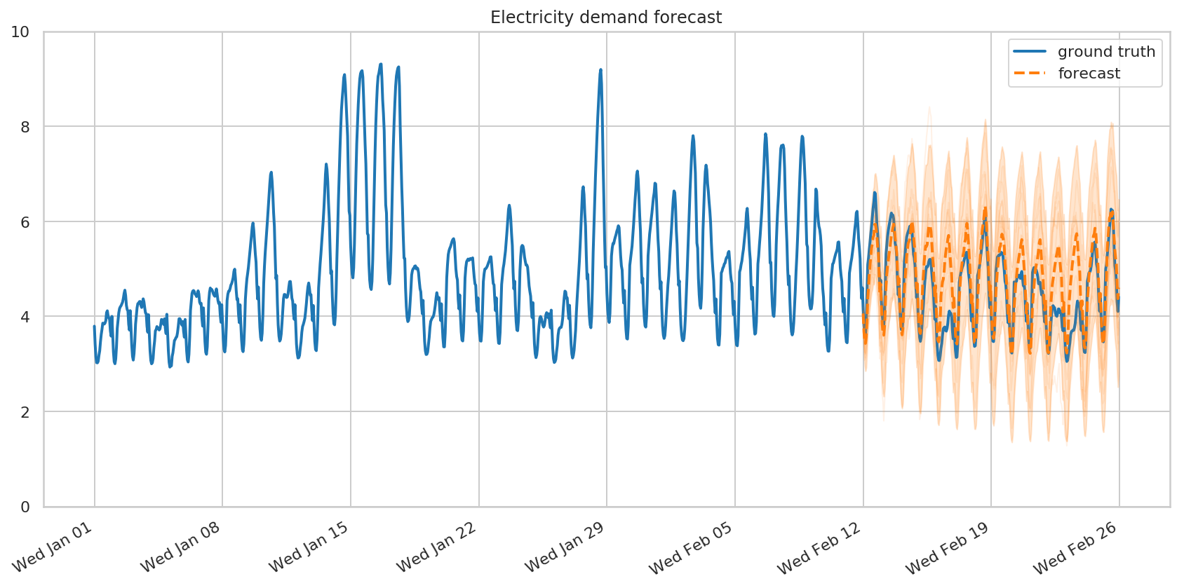
予測と批判
ここでも、モデル、時系列、およびサンプリングされたパラメーターを使用して tfp.sts.forecast を呼び出し、予測を作成します。
demand_forecast_dist = tfp.sts.forecast(
    model=demand_model,
    observed_time_series=demand_training_data,
    parameter_samples=q_samples_demand_,
    num_steps_forecast=num_forecast_steps)
num_samples=10

(
    demand_forecast_mean,
    demand_forecast_scale,
    demand_forecast_samples
) = (
    demand_forecast_dist.mean().numpy()[..., 0],
    demand_forecast_dist.stddev().numpy()[..., 0],
    demand_forecast_dist.sample(num_samples).numpy()[..., 0]
    )
fig, ax = plot_forecast(demand_dates, demand,
                        demand_forecast_mean,
                        demand_forecast_scale,
                        demand_forecast_samples,
                        title="Electricity demand forecast",
                        x_locator=demand_loc, x_formatter=demand_fmt)
ax.set_ylim([0, 10])
fig.tight_layout()
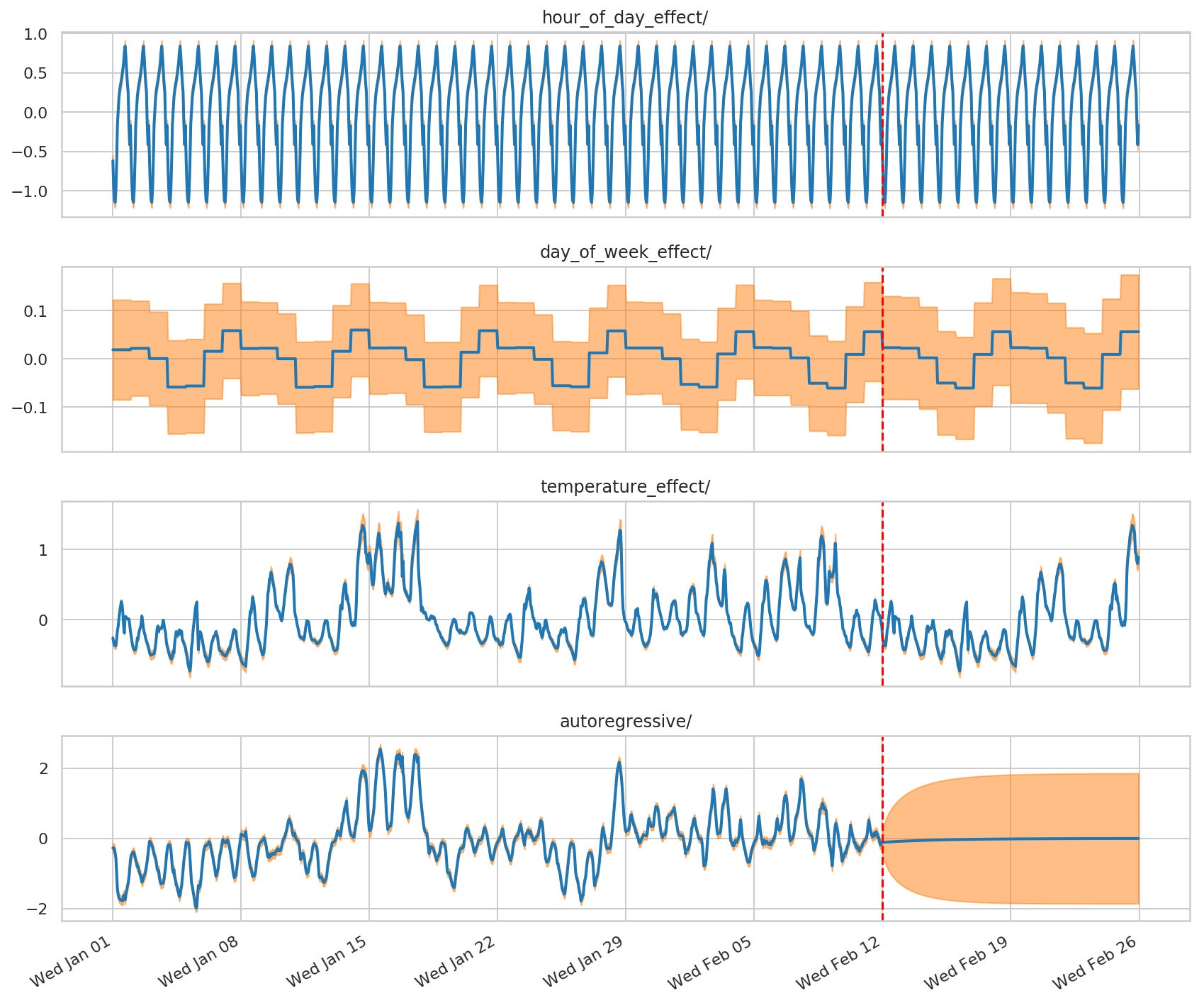
観測された系列と予測された系列の個々のコンポーネントへの分解を視覚化してみましょう。
# Get the distributions over component outputs from the posterior marginals on
# training data, and from the forecast model.
component_dists = sts.decompose_by_component(
    demand_model,
    observed_time_series=demand_training_data,
    parameter_samples=q_samples_demand_)

forecast_component_dists = sts.decompose_forecast_by_component(
    demand_model,
    forecast_dist=demand_forecast_dist,
    parameter_samples=q_samples_demand_)
demand_component_means_, demand_component_stddevs_ = (
    {k.name: c.mean() for k, c in component_dists.items()},
    {k.name: c.stddev() for k, c in component_dists.items()})

(
    demand_forecast_component_means_,
    demand_forecast_component_stddevs_
) = (
    {k.name: c.mean() for k, c in forecast_component_dists.items()},
    {k.name: c.stddev() for k, c in forecast_component_dists.items()}
    )
# Concatenate the training data with forecasts for plotting.
component_with_forecast_means_ = collections.OrderedDict()
component_with_forecast_stddevs_ = collections.OrderedDict()
for k in demand_component_means_.keys():
  component_with_forecast_means_[k] = np.concatenate([
      demand_component_means_[k],
      demand_forecast_component_means_[k]], axis=-1)
  component_with_forecast_stddevs_[k] = np.concatenate([
      demand_component_stddevs_[k],
      demand_forecast_component_stddevs_[k]], axis=-1)


fig, axes = plot_components(
  demand_dates,
  component_with_forecast_means_,
  component_with_forecast_stddevs_,
  x_locator=demand_loc, x_formatter=demand_fmt)
for ax in axes.values():
  ax.axvline(demand_dates[-num_forecast_steps], linestyle="--", color='red')
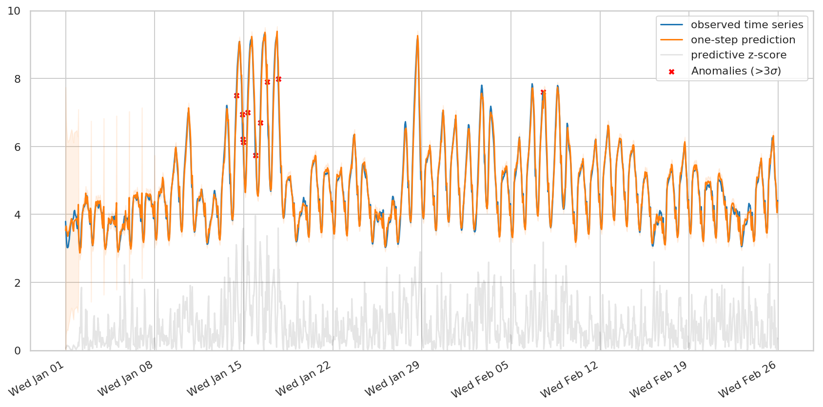
観測された系列の異常を検出するのであれば、ワンステップの予測分布、つまり、その時点までの時間ステップのみが与えられた場合の各時間ステップの予測にも関心があるかもしれません。 tfp.sts.one_step_predictive は、1回のパスで、すべてのワンステップ予測分布を計算します。
demand_one_step_dist = sts.one_step_predictive(
    demand_model,
    observed_time_series=demand,
    parameter_samples=q_samples_demand_)

demand_one_step_mean, demand_one_step_scale = (
    demand_one_step_dist.mean().numpy(), demand_one_step_dist.stddev().numpy())
単純な以上検出スキームは、観測が予測値の 3 つの stddev を超えるすべての時間ステップにフラグを立てることです。これらが、モデルによれば、最も「驚きのある」時間ステップです。
fig, ax = plot_one_step_predictive(
    demand_dates, demand,
    demand_one_step_mean, demand_one_step_scale,
    x_locator=demand_loc, x_formatter=demand_fmt)
ax.set_ylim(0, 10)

# Use the one-step-ahead forecasts to detect anomalous timesteps.
zscores = np.abs((demand - demand_one_step_mean) /
                 demand_one_step_scale)
anomalies = zscores > 3.0
ax.scatter(demand_dates[anomalies],
           demand[anomalies],
           c="red", marker="x", s=20, linewidth=2, label=r"Anomalies (>3$\sigma$)")
ax.plot(demand_dates, zscores, color="black", alpha=0.1, label='predictive z-score')
ax.legend()
plt.show()