
| |  GitHubでソースを表示 GitHubでソースを表示 | |
TensorFlow Quantumは、量子プリミティブをTensorFlowエコシステムにもたらします。現在、量子研究者はTensorFlowのツールを活用できます。このチュートリアルでは、 TensorBoardを量子コンピューティングの研究に組み込む方法について詳しく見ていきます。 TensorFlowのDCGANチュートリアルを使用すると、 Niu etalによって行われたものと同様の実用的な実験と視覚化をすばやく構築できます。 。大まかに言えば、次のようになります。
- 量子回路から来たように見えるサンプルを生成するようにGANをトレーニングします。
- トレーニングの進捗状況と、時間の経過に伴う分布の進化を視覚化します。
- 計算グラフを調べて、実験のベンチマークを行います。
pip install tensorflow==2.7.0 tensorflow-quantum tensorboard_plugin_profile==2.4.0
# Update package resources to account for version changes.
import importlib, pkg_resources
importlib.reload(pkg_resources)
<module 'pkg_resources' from '/tmpfs/src/tf_docs_env/lib/python3.7/site-packages/pkg_resources/__init__.py'>
#docs_infra: no_execute
%load_ext tensorboard
import datetime
import time
import cirq
import tensorflow as tf
import tensorflow_quantum as tfq
from tensorflow.keras import layers

# visualization tools
%matplotlib inline
import matplotlib.pyplot as plt
from cirq.contrib.svg import SVGCircuit
2022-02-04 12:46:52.770534: E tensorflow/stream_executor/cuda/cuda_driver.cc:271] failed call to cuInit: CUDA_ERROR_NO_DEVICE: no CUDA-capable device is detected
1.データ生成
いくつかのデータを収集することから始めます。 TensorFlow Quantumを使用して、残りの実験の主要なデータソースとなるビット文字列サンプルをすばやく生成できます。 Niuらのように。深さが大幅に減少したランダム回路からのサンプリングをエミュレートするのがいかに簡単かを探ります。まず、いくつかのヘルパーを定義します。
def generate_circuit(qubits):
    """Generate a random circuit on qubits."""
    random_circuit = cirq.generate_boixo_2018_supremacy_circuits_v2(
        qubits, cz_depth=2, seed=1234)
    return random_circuit

def generate_data(circuit, n_samples):
    """Draw n_samples samples from circuit into a tf.Tensor."""
    return tf.squeeze(tfq.layers.Sample()(circuit, repetitions=n_samples).to_tensor())
これで、回路といくつかのサンプルデータを検査できます。
qubits = cirq.GridQubit.rect(1, 5)
random_circuit_m = generate_circuit(qubits) + cirq.measure_each(*qubits)
SVGCircuit(random_circuit_m)
findfont: Font family ['Arial'] not found. Falling back to DejaVu Sans.

samples = cirq.sample(random_circuit_m, repetitions=10)
print('10 Random bitstrings from this circuit:')
print(samples)
10 Random bitstrings from this circuit:
(0, 0)=1000001000
(0, 1)=0000001010
(0, 2)=1010000100
(0, 3)=0010000110
(0, 4)=0110110010
TensorFlowQuantumでも同じことができます。
generate_data(random_circuit_m, 10)
<tf.Tensor: shape=(10, 5), dtype=int8, numpy=
array([[0, 0, 0, 0, 0],
       [0, 0, 0, 0, 0],
       [0, 0, 1, 0, 0],
       [0, 1, 0, 0, 0],
       [0, 1, 0, 0, 0],
       [0, 1, 1, 0, 0],
       [1, 0, 0, 0, 0],
       [1, 0, 0, 1, 0],
       [1, 1, 1, 0, 0],
       [1, 1, 1, 0, 0]], dtype=int8)>
これで、次の方法でトレーニングデータをすばやく生成できます。
N_SAMPLES = 60000
N_QUBITS = 10
QUBITS = cirq.GridQubit.rect(1, N_QUBITS)
REFERENCE_CIRCUIT = generate_circuit(QUBITS)
all_data = generate_data(REFERENCE_CIRCUIT, N_SAMPLES)
all_data
<tf.Tensor: shape=(60000, 10), dtype=int8, numpy=
array([[0, 0, 0, ..., 0, 0, 0],
       [0, 0, 0, ..., 0, 0, 0],
       [0, 0, 0, ..., 0, 0, 0],
       ...,
       [1, 1, 1, ..., 1, 1, 1],
       [1, 1, 1, ..., 1, 1, 1],
       [1, 1, 1, ..., 1, 1, 1]], dtype=int8)>
トレーニングが進行するにつれて視覚化するいくつかのヘルパー関数を定義すると便利です。使用する2つの興味深い量は次のとおりです。
- 分布のヒストグラムを作成できるように、サンプルの整数値。
- サンプルがどれほど「真に量子ランダム」であるかを示すための、サンプルセットの線形XEB忠実度推定。
@tf.function
def bits_to_ints(bits):
    """Convert tensor of bitstrings to tensor of ints."""
    sigs = tf.constant([1 << i for i in range(N_QUBITS)], dtype=tf.int32)
    rounded_bits = tf.clip_by_value(tf.math.round(
        tf.cast(bits, dtype=tf.dtypes.float32)), clip_value_min=0, clip_value_max=1)
    return tf.einsum('jk,k->j', tf.cast(rounded_bits, dtype=tf.dtypes.int32), sigs)

@tf.function
def xeb_fid(bits):
    """Compute linear XEB fidelity of bitstrings."""
    final_probs = tf.squeeze(
        tf.abs(tfq.layers.State()(REFERENCE_CIRCUIT).to_tensor()) ** 2)
    nums = bits_to_ints(bits)
    return (2 ** N_QUBITS) * tf.reduce_mean(tf.gather(final_probs, nums)) - 1.0
ここでは、XEBを使用して配布と健全性チェックを視覚化できます。
plt.hist(bits_to_ints(all_data).numpy(), 50)
plt.show()
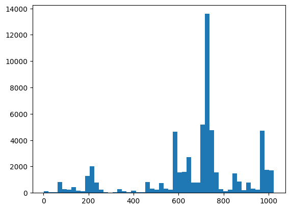
xeb_fid(all_data)
<tf.Tensor: shape=(), dtype=float32, numpy=-0.0015467405>プレースホルダー19
2.モデルを作成します
ここでは、クォンタムの場合のDCGANチュートリアルの関連コンポーネントを使用できます。 MNIST数字を生成する代わりに、新しいGANを使用して、長さN_QUBITSビット文字列サンプルを生成します。
LATENT_DIM = 100
def make_generator_model():
    """Construct generator model."""
    model = tf.keras.Sequential()
    model.add(layers.Dense(256, use_bias=False, input_shape=(LATENT_DIM,)))
    model.add(layers.Dense(128, activation='relu'))
    model.add(layers.Dropout(0.3))
    model.add(layers.Dense(64, activation='relu'))
    model.add(layers.Dense(N_QUBITS, activation='relu'))

    return model

def make_discriminator_model():
    """Constrcut discriminator model."""
    model = tf.keras.Sequential()
    model.add(layers.Dense(256, use_bias=False, input_shape=(N_QUBITS,)))
    model.add(layers.Dense(128, activation='relu'))
    model.add(layers.Dropout(0.3))
    model.add(layers.Dense(32, activation='relu'))
    model.add(layers.Dense(1))

    return model
次に、ジェネレーターとディスクリミネーターモデルをインスタンス化し、損失を定義し、メインのトレーニングループに使用するtrain_step関数を作成します。
discriminator = make_discriminator_model()
generator = make_generator_model()
cross_entropy = tf.keras.losses.BinaryCrossentropy(from_logits=True)
def discriminator_loss(real_output, fake_output):
    """Compute discriminator loss."""
    real_loss = cross_entropy(tf.ones_like(real_output), real_output)
    fake_loss = cross_entropy(tf.zeros_like(fake_output), fake_output)
    total_loss = real_loss + fake_loss
    return total_loss

def generator_loss(fake_output):
    """Compute generator loss."""
    return cross_entropy(tf.ones_like(fake_output), fake_output)

generator_optimizer = tf.keras.optimizers.Adam(1e-4)
discriminator_optimizer = tf.keras.optimizers.Adam(1e-4)
BATCH_SIZE=256

@tf.function
def train_step(images):
    """Run train step on provided image batch."""
    noise = tf.random.normal([BATCH_SIZE, LATENT_DIM])
    with tf.GradientTape() as gen_tape, tf.GradientTape() as disc_tape:
        generated_images = generator(noise, training=True)

        real_output = discriminator(images, training=True)
        fake_output = discriminator(generated_images, training=True)

        gen_loss = generator_loss(fake_output)
        disc_loss = discriminator_loss(real_output, fake_output)

    gradients_of_generator = gen_tape.gradient(
        gen_loss, generator.trainable_variables)
    gradients_of_discriminator = disc_tape.gradient(
        disc_loss, discriminator.trainable_variables)

    generator_optimizer.apply_gradients(
        zip(gradients_of_generator, generator.trainable_variables))
    discriminator_optimizer.apply_gradients(
        zip(gradients_of_discriminator, discriminator.trainable_variables))

    return gen_loss, disc_loss
モデルに必要なすべてのビルディングブロックが揃ったので、TensorBoardの視覚化を組み込んだトレーニング関数を設定できます。最初にTensorBoardファイルライターをセットアップします。
logdir = "tb_logs/" + datetime.datetime.now().strftime("%Y%m%d-%H%M%S")
file_writer = tf.summary.create_file_writer(logdir + "/metrics")
file_writer.set_as_default()
tf.summaryモジュールを使用して、メインtrain関数内のTensorBoardにscalar 、 histogram (およびその他)のログを組み込むことができるようになりました。
def train(dataset, epochs, start_epoch=1):
    """Launch full training run for the given number of epochs."""
    # Log original training distribution.
    tf.summary.histogram('Training Distribution', data=bits_to_ints(dataset), step=0)

    batched_data = tf.data.Dataset.from_tensor_slices(dataset).shuffle(N_SAMPLES).batch(512)
    t = time.time()
    for epoch in range(start_epoch, start_epoch + epochs):
        for i, image_batch in enumerate(batched_data):
            # Log batch-wise loss.
            gl, dl = train_step(image_batch)
            tf.summary.scalar(
                'Generator loss', data=gl, step=epoch * len(batched_data) + i)
            tf.summary.scalar(
                'Discriminator loss', data=dl, step=epoch * len(batched_data) + i)

        # Log full dataset XEB Fidelity and generated distribution.
        generated_samples = generator(tf.random.normal([N_SAMPLES, 100]))
        tf.summary.scalar(
        'Generator XEB Fidelity Estimate', data=xeb_fid(generated_samples), step=epoch)
        tf.summary.histogram(
        'Generator distribution', data=bits_to_ints(generated_samples), step=epoch)
        # Log new samples drawn from this particular random circuit.
        random_new_distribution = generate_data(REFERENCE_CIRCUIT, N_SAMPLES)
        tf.summary.histogram(
        'New round of True samples', data=bits_to_ints(random_new_distribution), step=epoch)

        if epoch % 10 == 0:
            print('Epoch {}, took {}(s)'.format(epoch, time.time() - t))
            t = time.time()
3.トレーニングとパフォーマンスを視覚化する
TensorBoardダッシュボードは次のコマンドで起動できるようになりました。
#docs_infra: no_execute
%tensorboard --logdir tb_logs/
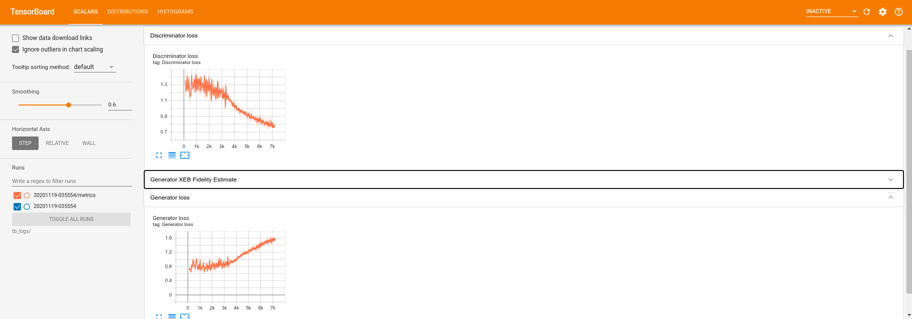
trainを呼び出すと、TensoBoardダッシュボードは、トレーニングループで指定されたすべての要約統計量で自動更新されます。
train(all_data, epochs=50)
Epoch 10, took 9.325464487075806(s)
Epoch 20, took 7.684147119522095(s)
Epoch 30, took 7.508770704269409(s)
Epoch 40, took 7.5157341957092285(s)
Epoch 50, took 7.533370494842529(s)
プレースホルダー28
トレーニングの実行中(およびトレーニングが完了すると)、スカラー量を調べることができます。
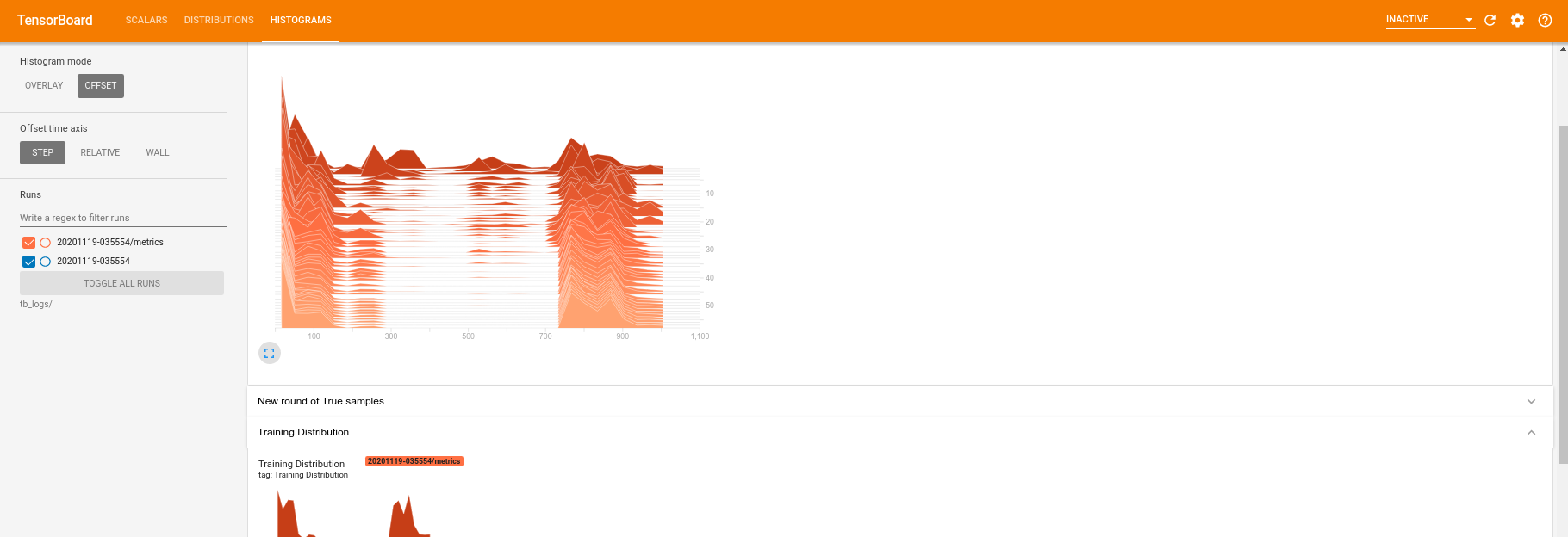
[ヒストグラム]タブに切り替えると、量子分布からサンプルを再作成する際にジェネレーターネットワークがどの程度うまく機能しているかを確認することもできます。
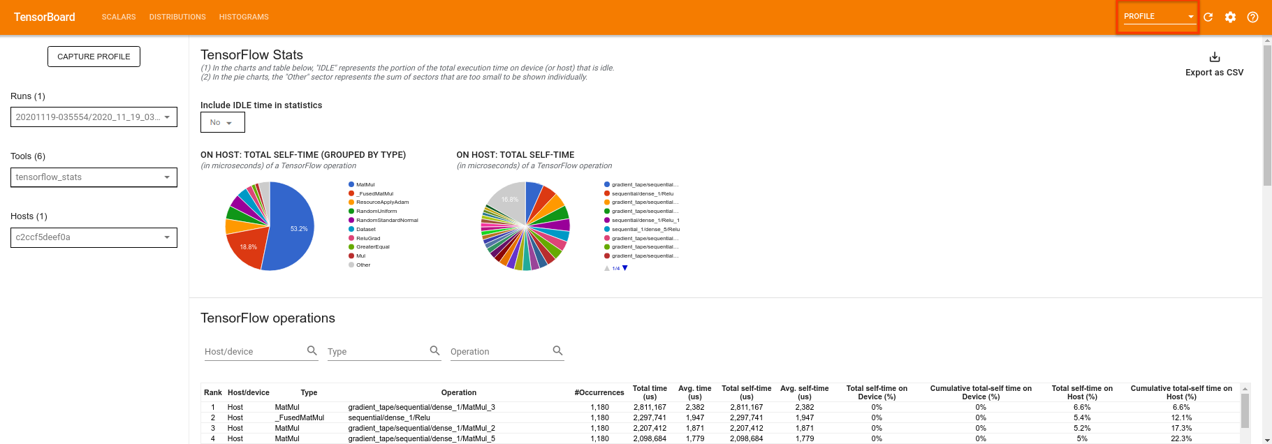
TensorBoardは、実験に関連する要約統計量のリアルタイムモニタリングを可能にするだけでなく、パフォーマンスのボトルネックを特定するために実験のプロファイルを作成するのにも役立ちます。パフォーマンスモニタリングを使用してモデルを再実行するには、次の操作を実行できます。
tf.profiler.experimental.start(logdir)
train(all_data, epochs=10, start_epoch=50)
tf.profiler.experimental.stop()
Epoch 50, took 0.8879530429840088(s)
TensorBoardは、 tf.profiler.experimental.startとtf.profiler.experimental.stopの間のすべてのコードをプロファイリングします。このプロファイルデータは、TensorBoardのprofileページで表示できます。
深さを増やすか、さまざまなクラスの量子回路を試してみてください。 TensorFlow Quantum実験に組み込むことができるハイパーパラメータ調整など、 TensorBoardの他のすべての優れた機能を確認してください。