
| | |  צפה במקור ב-GitHub צפה במקור ב-GitHub | |
סקירה כללית
השימוש ב- API סיכום תמונת TensorFlow, אתה יכול להתחבר tensors בקלות ותמונות שרירותיות ולהציג אותם TensorBoard. זה יכול להיות מועיל מאוד לטעום ולבחון נתוני הקלט שלך, או כדי להמחיש משקולות שכבת ו tensors שנוצר . אתה יכול גם לרשום נתוני אבחון כתמונות שיכולות להיות מועילות במהלך פיתוח המודל שלך.
במדריך זה, תלמד כיצד להשתמש ב-API של סיכום תמונה כדי להמחיש טנסורים כתמונות. תלמדו גם איך לצלם תמונה שרירותית, להמיר אותה לטנזור ולדמיין אותה ב- TensorBoard. תעבדו על דוגמה פשוטה אך אמיתית המשתמשת בסיכומי תמונה כדי לעזור לכם להבין כיצד המודל שלכם מתפקד.
להכין
try:
  # %tensorflow_version only exists in Colab.
  %tensorflow_version 2.x
except Exception:
  pass

# Load the TensorBoard notebook extension.
%load_ext tensorboard
TensorFlow 2.x selected.
from datetime import datetime
import io
import itertools
from packaging import version

import tensorflow as tf
from tensorflow import keras

import matplotlib.pyplot as plt
import numpy as np
import sklearn.metrics

print("TensorFlow version: ", tf.__version__)
assert version.parse(tf.__version__).release[0] >= 2, \
    "This notebook requires TensorFlow 2.0 or above."
TensorFlow version: 2.2
הורד את מערך הנתונים של Fashion-MNIST
אתה הולך לבנות רשת עצבית פשוט תמונות לסווג באזור סמוך לבית האופנה-MNIST נתון. מערך נתונים זה מורכב מ-70,000 תמונות בגווני אפור בגודל 28x28 של מוצרי אופנה מ-10 קטגוריות, עם 7,000 תמונות לכל קטגוריה.
ראשית, הורד את הנתונים:
# Download the data. The data is already divided into train and test.
# The labels are integers representing classes.
fashion_mnist = keras.datasets.fashion_mnist
(train_images, train_labels), (test_images, test_labels) = \
    fashion_mnist.load_data()

# Names of the integer classes, i.e., 0 -> T-short/top, 1 -> Trouser, etc.
class_names = ['T-shirt/top', 'Trouser', 'Pullover', 'Dress', 'Coat',
    'Sandal', 'Shirt', 'Sneaker', 'Bag', 'Ankle boot']
Downloading data from https://storage.googleapis.com/tensorflow/tf-keras-datasets/train-labels-idx1-ubyte.gz
32768/29515 [=================================] - 0s 0us/step
Downloading data from https://storage.googleapis.com/tensorflow/tf-keras-datasets/train-images-idx3-ubyte.gz
26427392/26421880 [==============================] - 0s 0us/step
Downloading data from https://storage.googleapis.com/tensorflow/tf-keras-datasets/t10k-labels-idx1-ubyte.gz
8192/5148 [===============================================] - 0s 0us/step
Downloading data from https://storage.googleapis.com/tensorflow/tf-keras-datasets/t10k-images-idx3-ubyte.gz
4423680/4422102 [==============================] - 0s 0us/step
הדמיית תמונה בודדת
כדי להבין כיצד פועל ממשק ה-API של Image Summary, כעת אתה פשוט הולך לרשום את תמונת האימון הראשונה בערכת האימונים שלך ב-TensorBoard.
לפני שתעשה זאת, בדוק את צורת נתוני האימון שלך:
print("Shape: ", train_images[0].shape)
print("Label: ", train_labels[0], "->", class_names[train_labels[0]])
Shape:  (28, 28)
Label:  9 -> Ankle boot
שימו לב שהצורה של כל תמונה במערך הנתונים היא טנסור צורה בדרגה 2 (28, 28), המייצג את הגובה והרוחב.
עם זאת, tf.summary.image() מצפה מותח דרגה-4 המכיל (batch_size, height, width, channels) . לכן, יש לעצב מחדש את הטנסורים.
אתה רישום רחוק רק תמונה אחת, כך batch_size הוא 1. התמונות הן בגוונים אפורות, לכן קבעת channels אל 1.
# Reshape the image for the Summary API.
img = np.reshape(train_images[0], (-1, 28, 28, 1))
כעת אתה מוכן לרשום את התמונה הזו ולהציג אותה ב-TensorBoard.
# Clear out any prior log data.
!rm -rf logs

# Sets up a timestamped log directory.
logdir = "logs/train_data/" + datetime.now().strftime("%Y%m%d-%H%M%S")
# Creates a file writer for the log directory.
file_writer = tf.summary.create_file_writer(logdir)

# Using the file writer, log the reshaped image.
with file_writer.as_default():
  tf.summary.image("Training data", img, step=0)
כעת, השתמש ב- TensorBoard כדי לבחון את התמונה. המתן מספר שניות עד שממשק המשתמש יתהפך.
%tensorboard --logdir logs/train_data

הכרטיסייה "תמונות" מציגה את התמונה שזה עתה רשמת. זה "מגפון קרסול".
קנה המידה של התמונה לגודל ברירת מחדל לצפייה קלה יותר. אם ברצונך להציג את התמונה המקורית ללא קנה מידה, סמן את "הצג גודל תמונה בפועל" בפינה השמאלית העליונה.
שחקו עם מחווני הבהירות והניגודיות כדי לראות כיצד הם משפיעים על פיקסלים של התמונה.
הדמיית תמונות מרובות
רישום טנזור אחד הוא נהדר, אבל מה אם תרצה לרשום דוגמאות מרובות לאימון?
כל שעליך לעשות הוא לציין את מספר התמונות שאתה רוצה להתחבר כאשר העברת הנתונים tf.summary.image() .
with file_writer.as_default():
  # Don't forget to reshape.
  images = np.reshape(train_images[0:25], (-1, 28, 28, 1))
  tf.summary.image("25 training data examples", images, max_outputs=25, step=0)

%tensorboard --logdir logs/train_data

רישום נתוני תמונה שרירותיים
מה אם אתה רוצה לדמיין תמונה לא מותח, כגון דימוי שנוצר על ידי matplotlib ?
אתה צריך קוד לוח כדי להמיר את העלילה לטנזור, אבל אחרי זה, אתה מוכן ללכת.
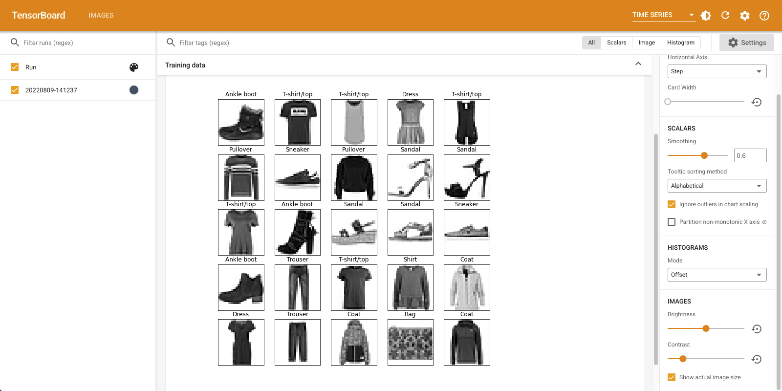
בקוד שלמטה, תוכל להיכנס 25 התמונות הראשונות כרשת נחמדת באמצעות של matplotlib subplot() פונקציה. לאחר מכן תראה את הרשת ב-TensorBoard:
# Clear out prior logging data.
!rm -rf logs/plots

logdir = "logs/plots/" + datetime.now().strftime("%Y%m%d-%H%M%S")
file_writer = tf.summary.create_file_writer(logdir)

def plot_to_image(figure):
  """Converts the matplotlib plot specified by 'figure' to a PNG image and
  returns it. The supplied figure is closed and inaccessible after this call."""
  # Save the plot to a PNG in memory.
  buf = io.BytesIO()
  plt.savefig(buf, format='png')
  # Closing the figure prevents it from being displayed directly inside
  # the notebook.
  plt.close(figure)
  buf.seek(0)
  # Convert PNG buffer to TF image
  image = tf.image.decode_png(buf.getvalue(), channels=4)
  # Add the batch dimension
  image = tf.expand_dims(image, 0)
  return image

def image_grid():
  """Return a 5x5 grid of the MNIST images as a matplotlib figure."""
  # Create a figure to contain the plot.
  figure = plt.figure(figsize=(10,10))
  for i in range(25):
    # Start next subplot.
    plt.subplot(5, 5, i + 1, title=class_names[train_labels[i]])
    plt.xticks([])
    plt.yticks([])
    plt.grid(False)
    plt.imshow(train_images[i], cmap=plt.cm.binary)

  return figure

# Prepare the plot
figure = image_grid()
# Convert to image and log
with file_writer.as_default():
  tf.summary.image("Training data", plot_to_image(figure), step=0)

%tensorboard --logdir logs/plots
בניית סיווג תמונה
עכשיו חבר את כל זה יחד עם דוגמה אמיתית. אחרי הכל, אתה כאן כדי לעשות למידת מכונה ולא לתכנן תמונות יפות!
אתה הולך להשתמש בסיכומי תמונות כדי להבין עד כמה המודל שלך מצליח בזמן אימון מסווג פשוט עבור מערך הנתונים של Fashion-MNIST.
ראשית, צור מודל פשוט מאוד והידור אותו, הגדר את פונקציית האופטימיזציה וההפסד. שלב ההידור גם מציין שברצונך לרשום את הדיוק של המסווג לאורך הדרך.
model = keras.models.Sequential([
    keras.layers.Flatten(input_shape=(28, 28)),
    keras.layers.Dense(32, activation='relu'),
    keras.layers.Dense(10, activation='softmax')
])

model.compile(
    optimizer='adam',
    loss='sparse_categorical_crossentropy',
    metrics=['accuracy']
)
כאשר מתאמנים מסווג, זה שימושי כדי לראות את מטריקס הבלבול . מטריצת הבלבול מעניקה לך ידע מפורט על הביצועים של המסווג שלך בנתוני הבדיקה.
הגדר פונקציה שמחשבת את מטריצת הבלבול. תוכל להשתמש נוח Scikit-ללמוד פונקציה שעושה זאת, ולאחר מכן לשרטט אותו באמצעות matplotlib.
def plot_confusion_matrix(cm, class_names):
  """
  Returns a matplotlib figure containing the plotted confusion matrix.

  Args:
    cm (array, shape = [n, n]): a confusion matrix of integer classes
    class_names (array, shape = [n]): String names of the integer classes
  """
  figure = plt.figure(figsize=(8, 8))
  plt.imshow(cm, interpolation='nearest', cmap=plt.cm.Blues)
  plt.title("Confusion matrix")
  plt.colorbar()
  tick_marks = np.arange(len(class_names))
  plt.xticks(tick_marks, class_names, rotation=45)
  plt.yticks(tick_marks, class_names)

  # Compute the labels from the normalized confusion matrix.
  labels = np.around(cm.astype('float') / cm.sum(axis=1)[:, np.newaxis], decimals=2)

  # Use white text if squares are dark; otherwise black.
  threshold = cm.max() / 2.
  for i, j in itertools.product(range(cm.shape[0]), range(cm.shape[1])):
    color = "white" if cm[i, j] > threshold else "black"
    plt.text(j, i, labels[i, j], horizontalalignment="center", color=color)

  plt.tight_layout()
  plt.ylabel('True label')
  plt.xlabel('Predicted label')
  return figure
כעת אתה מוכן לאמן את המסווגן ולרשום באופן קבוע את מטריצת הבלבול לאורך הדרך.
הנה מה שתעשה:
- צור את התקשרות Keras TensorBoard להיכנס מדדים בסיסיים
- צור Keras LambdaCallback להיכנס מטריצת בלבול בסוף כל תקופה
- אמן את המודל באמצעות Model.fit(), תוך הקפדה על העברה של שתי ההתקשרויות
ככל שהאימון מתקדם, גלול מטה כדי לראות את TensorBoard מופעל.
# Clear out prior logging data.
!rm -rf logs/image

logdir = "logs/image/" + datetime.now().strftime("%Y%m%d-%H%M%S")
# Define the basic TensorBoard callback.
tensorboard_callback = keras.callbacks.TensorBoard(log_dir=logdir)
file_writer_cm = tf.summary.create_file_writer(logdir + '/cm')
def log_confusion_matrix(epoch, logs):
  # Use the model to predict the values from the validation dataset.
  test_pred_raw = model.predict(test_images)
  test_pred = np.argmax(test_pred_raw, axis=1)

  # Calculate the confusion matrix.
  cm = sklearn.metrics.confusion_matrix(test_labels, test_pred)
  # Log the confusion matrix as an image summary.
  figure = plot_confusion_matrix(cm, class_names=class_names)
  cm_image = plot_to_image(figure)

  # Log the confusion matrix as an image summary.
  with file_writer_cm.as_default():
    tf.summary.image("Confusion Matrix", cm_image, step=epoch)

# Define the per-epoch callback.
cm_callback = keras.callbacks.LambdaCallback(on_epoch_end=log_confusion_matrix)
# Start TensorBoard.
%tensorboard --logdir logs/image

# Train the classifier.
model.fit(
    train_images,
    train_labels,
    epochs=5,
    verbose=0, # Suppress chatty output
    callbacks=[tensorboard_callback, cm_callback],
    validation_data=(test_images, test_labels),
)
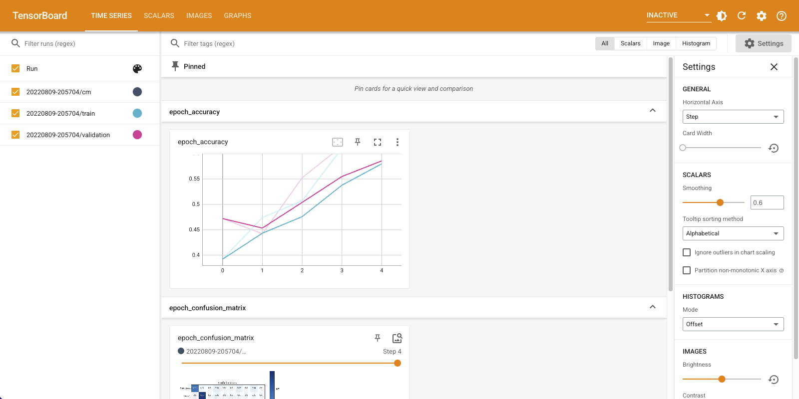
שימו לב שהדיוק מטפס הן בערכות הרכבת והן בערכות האימות. זה סימן טוב. אבל איך המודל מתפקד על תת-קבוצות ספציפיות של הנתונים?
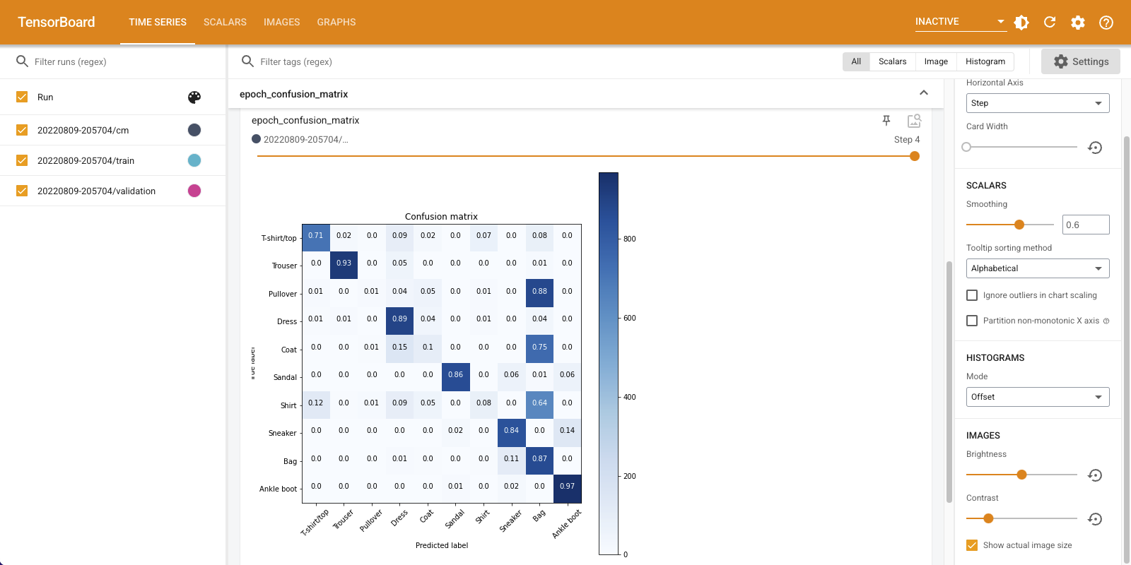
בחר בכרטיסייה "תמונות" כדי לדמיין את מטריצות הבלבול הרשומות שלך. סמן את "הצג גודל תמונה בפועל" בפינה השמאלית העליונה כדי לראות את מטריצת הבלבול בגודל מלא.
כברירת מחדל, לוח המחוונים מציג את סיכום התמונה עבור השלב האחרון או התקופה שנרשמה. השתמש במחוון כדי להציג מטריצות בלבול קודמות. שימו לב כיצד המטריצה משתנה באופן משמעותי ככל שהאימון מתקדם, כאשר ריבועים כהים יותר מתלכדים לאורך האלכסון, ושאר המטריצה נוטה לכיוון 0 ולבן. זה אומר שהמסווג שלך משתפר ככל שהאימונים מתקדמים! עבודה נהדרת!
מטריצת הבלבול מראה שלמודל הפשוט הזה יש כמה בעיות. למרות ההתקדמות הגדולה, חולצות, חולצות טריקו וסוודרים מתבלבלים זה עם זה. הדגם צריך עוד עבודה.
אם אתה מעוניין, לנסות לשפר את המודל הזה עם רשת קונבולוציה (CNN).