
| |
|
 GitHub でソースを表示 GitHub でソースを表示 |
TF-Hub は、機械学習の知識を再利用可能なリソース、特にトレーニング済みのモジュールとしてパッケージ化した知識を共有するためのプラットフォームです。このチュートリアルでは、TF-Hub テキスト埋め込みモジュールを使用して、合理的なベースラインの精度による単純なセンチメント分類器のトレーニングを行います。その後で、予測を Kaggle に送信します。
TF-Hub によるテキスト分類と精度を改善するための追加手順に関する詳細なチュートリアルについては、TF-Hub によるテキスト分類をご覧ください。
セットアップ
pip install -q kaggleimport tensorflow as tf
import tensorflow_hub as hub
import matplotlib.pyplot as plt
import numpy as np
import pandas as pd
import seaborn as sns
import zipfile
from sklearn import model_selection
2024-01-11 18:11:46.618840: E external/local_xla/xla/stream_executor/cuda/cuda_dnn.cc:9261] Unable to register cuDNN factory: Attempting to register factory for plugin cuDNN when one has already been registered
2024-01-11 18:11:46.618891: E external/local_xla/xla/stream_executor/cuda/cuda_fft.cc:607] Unable to register cuFFT factory: Attempting to register factory for plugin cuFFT when one has already been registered
2024-01-11 18:11:46.620476: E external/local_xla/xla/stream_executor/cuda/cuda_blas.cc:1515] Unable to register cuBLAS factory: Attempting to register factory for plugin cuBLAS when one has already been registered
このチュートリアルでは Kaggle のデータセットを使用するため、Kaggle アカウントの API トークンの作成と、Colab 環境へのトークンのアップロードが必要となります。
import os
import pathlib

# Upload the API token.
def get_kaggle():
  try:
    import kaggle
    return kaggle
  except OSError:
    pass

  token_file = pathlib.Path("~/.kaggle/kaggle.json").expanduser()
  token_file.parent.mkdir(exist_ok=True, parents=True)

  try:
    from google.colab import files
  except ImportError:
    raise ValueError("Could not find kaggle token.")

  uploaded = files.upload()
  token_content = uploaded.get('kaggle.json', None)
  if token_content:
    token_file.write_bytes(token_content)
    token_file.chmod(0o600)
  else:
    raise ValueError('Need a file named "kaggle.json"')

  import kaggle
  return kaggle


kaggle = get_kaggle()
はじめに
データ
Kaggle の Sentiment Analysis on Movie Reviews(映画レビューのセンチメント分析)タスクを解いてみましょう。データセットには、Rotten Tomatoes という映画のレビューの構文サブフレーズが含まれます。これは、フレーズを 1 から 5 の段階で negative(否定的)または positive(肯定的)にラベル付けするタスクです。
API を使用してデータをダウンロードする前に、コンペのルールに同意する必要があります。
SENTIMENT_LABELS = [
    "negative", "somewhat negative", "neutral", "somewhat positive", "positive"
]

# Add a column with readable values representing the sentiment.
def add_readable_labels_column(df, sentiment_value_column):
  df["SentimentLabel"] = df[sentiment_value_column].replace(
      range(5), SENTIMENT_LABELS)

# Download data from Kaggle and create a DataFrame.
def load_data_from_zip(path):
  with zipfile.ZipFile(path, "r") as zip_ref:
    name = zip_ref.namelist()[0]
    with zip_ref.open(name) as zf:
      return pd.read_csv(zf, sep="\t", index_col=0)


# The data does not come with a validation set so we'll create one from the
# training set.
def get_data(competition, train_file, test_file, validation_set_ratio=0.1):
  data_path = pathlib.Path("data")
  kaggle.api.competition_download_files(competition, data_path)
  competition_path = (data_path/competition)
  competition_path.mkdir(exist_ok=True, parents=True)
  competition_zip_path = competition_path.with_suffix(".zip")

  with zipfile.ZipFile(competition_zip_path, "r") as zip_ref:
    zip_ref.extractall(competition_path)

  train_df = load_data_from_zip(competition_path/train_file)
  test_df = load_data_from_zip(competition_path/test_file)

  # Add a human readable label.
  add_readable_labels_column(train_df, "Sentiment")

  # We split by sentence ids, because we don't want to have phrases belonging
  # to the same sentence in both training and validation set.
  train_indices, validation_indices = model_selection.train_test_split(
      np.unique(train_df["SentenceId"]),
      test_size=validation_set_ratio,
      random_state=0)

  validation_df = train_df[train_df["SentenceId"].isin(validation_indices)]
  train_df = train_df[train_df["SentenceId"].isin(train_indices)]
  print("Split the training data into %d training and %d validation examples." %
        (len(train_df), len(validation_df)))

  return train_df, validation_df, test_df


train_df, validation_df, test_df = get_data(
    "sentiment-analysis-on-movie-reviews",
    "train.tsv.zip", "test.tsv.zip")
Split the training data into 140315 training and 15745 validation examples.
注意: このコンペのタスクは、すべてのレビューではなく、レビュー内の個別のフレーズを評価することで、難易度の非常に高いタスクと言えます。
train_df.head(20)
モデルをトレーニングする
注意: このタスクは回帰としてもモデル化することが可能です。TF-Hub によるテキスト分類をご覧ください。
class MyModel(tf.keras.Model):
  def __init__(self, hub_url):
    super().__init__()
    self.hub_url = hub_url
    self.embed = hub.load(self.hub_url).signatures['default']
    self.sequential = tf.keras.Sequential([
      tf.keras.layers.Dense(500),
      tf.keras.layers.Dense(100),
      tf.keras.layers.Dense(5),
    ])

  def call(self, inputs):
    phrases = inputs['Phrase'][:,0]
    embedding = 5*self.embed(phrases)['default']
    return self.sequential(embedding)

  def get_config(self):
    return {"hub_url":self.hub_url}
model = MyModel("https://tfhub.dev/google/nnlm-en-dim128/1")
model.compile(
    loss = tf.losses.SparseCategoricalCrossentropy(from_logits=True),
    optimizer=tf.optimizers.Adam(),
    metrics = [tf.keras.metrics.SparseCategoricalAccuracy(name="accuracy")])
history = model.fit(x=dict(train_df), y=train_df['Sentiment'],
          validation_data=(dict(validation_df), validation_df['Sentiment']),
          epochs = 25)
Epoch 1/25
WARNING: All log messages before absl::InitializeLog() is called are written to STDERR
I0000 00:00:1704996720.969617   33600 device_compiler.h:186] Compiled cluster using XLA!  This line is logged at most once for the lifetime of the process.
4385/4385 [==============================] - 15s 3ms/step - loss: 1.0242 - accuracy: 0.5864 - val_loss: 1.0005 - val_accuracy: 0.5820
Epoch 2/25
4385/4385 [==============================] - 13s 3ms/step - loss: 0.9998 - accuracy: 0.5944 - val_loss: 0.9953 - val_accuracy: 0.5916
Epoch 3/25
4385/4385 [==============================] - 13s 3ms/step - loss: 0.9952 - accuracy: 0.5961 - val_loss: 0.9850 - val_accuracy: 0.5968
Epoch 4/25
4385/4385 [==============================] - 13s 3ms/step - loss: 0.9924 - accuracy: 0.5978 - val_loss: 0.9881 - val_accuracy: 0.5943
Epoch 5/25
4385/4385 [==============================] - 13s 3ms/step - loss: 0.9915 - accuracy: 0.5977 - val_loss: 0.9796 - val_accuracy: 0.5966
Epoch 6/25
4385/4385 [==============================] - 14s 3ms/step - loss: 0.9904 - accuracy: 0.5988 - val_loss: 0.9834 - val_accuracy: 0.5968
Epoch 7/25
4385/4385 [==============================] - 13s 3ms/step - loss: 0.9892 - accuracy: 0.5991 - val_loss: 0.9807 - val_accuracy: 0.5921
Epoch 8/25
4385/4385 [==============================] - 13s 3ms/step - loss: 0.9890 - accuracy: 0.5994 - val_loss: 0.9817 - val_accuracy: 0.5971
Epoch 9/25
4385/4385 [==============================] - 13s 3ms/step - loss: 0.9883 - accuracy: 0.5993 - val_loss: 0.9828 - val_accuracy: 0.5970
Epoch 10/25
4385/4385 [==============================] - 13s 3ms/step - loss: 0.9878 - accuracy: 0.5992 - val_loss: 0.9781 - val_accuracy: 0.6011
Epoch 11/25
4385/4385 [==============================] - 13s 3ms/step - loss: 0.9877 - accuracy: 0.5989 - val_loss: 0.9886 - val_accuracy: 0.5933
Epoch 12/25
4385/4385 [==============================] - 13s 3ms/step - loss: 0.9874 - accuracy: 0.5992 - val_loss: 0.9778 - val_accuracy: 0.5940
Epoch 13/25
4385/4385 [==============================] - 13s 3ms/step - loss: 0.9872 - accuracy: 0.5991 - val_loss: 0.9809 - val_accuracy: 0.5945
Epoch 14/25
4385/4385 [==============================] - 13s 3ms/step - loss: 0.9866 - accuracy: 0.6006 - val_loss: 0.9841 - val_accuracy: 0.6017
Epoch 15/25
4385/4385 [==============================] - 13s 3ms/step - loss: 0.9869 - accuracy: 0.5990 - val_loss: 0.9816 - val_accuracy: 0.5943
Epoch 16/25
4385/4385 [==============================] - 13s 3ms/step - loss: 0.9866 - accuracy: 0.5989 - val_loss: 0.9819 - val_accuracy: 0.5939
Epoch 17/25
4385/4385 [==============================] - 13s 3ms/step - loss: 0.9862 - accuracy: 0.6000 - val_loss: 0.9816 - val_accuracy: 0.5942
Epoch 18/25
4385/4385 [==============================] - 13s 3ms/step - loss: 0.9864 - accuracy: 0.5998 - val_loss: 0.9817 - val_accuracy: 0.5978
Epoch 19/25
4385/4385 [==============================] - 13s 3ms/step - loss: 0.9861 - accuracy: 0.6007 - val_loss: 0.9790 - val_accuracy: 0.5972
Epoch 20/25
4385/4385 [==============================] - 13s 3ms/step - loss: 0.9863 - accuracy: 0.5991 - val_loss: 0.9800 - val_accuracy: 0.5942
Epoch 21/25
4385/4385 [==============================] - 13s 3ms/step - loss: 0.9859 - accuracy: 0.5999 - val_loss: 0.9823 - val_accuracy: 0.5920
Epoch 22/25
4385/4385 [==============================] - 13s 3ms/step - loss: 0.9858 - accuracy: 0.6004 - val_loss: 0.9819 - val_accuracy: 0.5931
Epoch 23/25
4385/4385 [==============================] - 13s 3ms/step - loss: 0.9859 - accuracy: 0.5997 - val_loss: 0.9772 - val_accuracy: 0.5970
Epoch 24/25
4385/4385 [==============================] - 13s 3ms/step - loss: 0.9858 - accuracy: 0.6004 - val_loss: 0.9882 - val_accuracy: 0.5877
Epoch 25/25
4385/4385 [==============================] - 13s 3ms/step - loss: 0.9856 - accuracy: 0.5996 - val_loss: 0.9800 - val_accuracy: 0.5963
予測
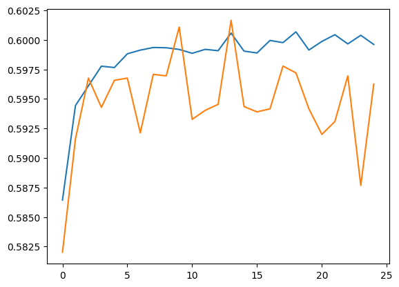
検証セットとトレーニングセットの予測を実行します。
plt.plot(history.history['accuracy'])
plt.plot(history.history['val_accuracy'])
[<matplotlib.lines.Line2D at 0x7f59561a35b0>]
train_eval_result = model.evaluate(dict(train_df), train_df['Sentiment'])
validation_eval_result = model.evaluate(dict(validation_df), validation_df['Sentiment'])

print(f"Training set accuracy: {train_eval_result[1]}")
print(f"Validation set accuracy: {validation_eval_result[1]}")
4385/4385 [==============================] - 13s 3ms/step - loss: 0.9833 - accuracy: 0.6009
493/493 [==============================] - 1s 2ms/step - loss: 0.9800 - accuracy: 0.5963
Training set accuracy: 0.6009407639503479
Validation set accuracy: 0.5962527990341187
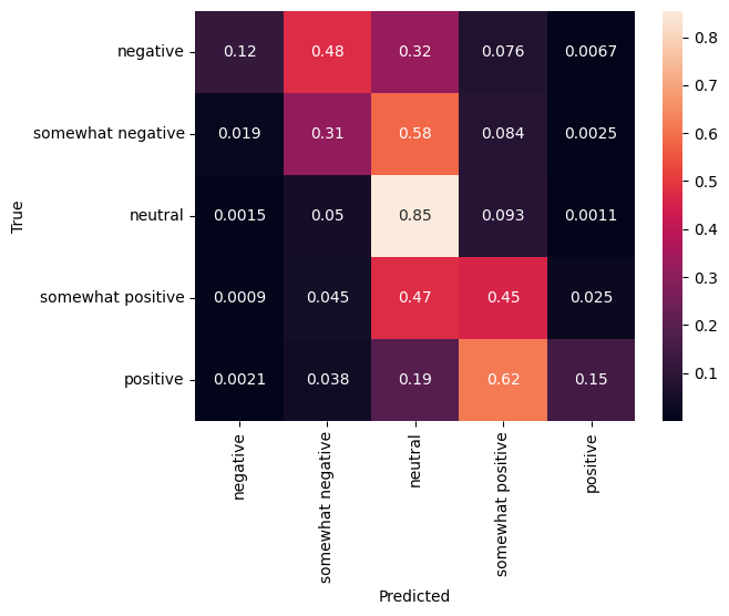
混同行列
特にマルチクラスの問題におけるもう 1 つの非常に興味深い統計に、混同行列というのがあります。混同行列では、正確および不正確にラベル付けされたサンプルの比率を視覚化することができます。そのため、分類器がどの程度偏っているのか、ラベルの分布に意味があるかどうかを簡単に確認することができます。予測の最大部分が対角線に沿って分散されているのが理想です。
predictions = model.predict(dict(validation_df))
predictions = tf.argmax(predictions, axis=-1)
predictions
493/493 [==============================] - 1s 2ms/step
<tf.Tensor: shape=(15745,), dtype=int64, numpy=array([1, 1, 2, ..., 2, 2, 2])>
cm = tf.math.confusion_matrix(validation_df['Sentiment'], predictions)
cm = cm/cm.numpy().sum(axis=1)[:, tf.newaxis]
sns.heatmap(
    cm, annot=True,
    xticklabels=SENTIMENT_LABELS,
    yticklabels=SENTIMENT_LABELS)
plt.xlabel("Predicted")
plt.ylabel("True")
Text(50.72222222222221, 0.5, 'True')
次のコードをコードセルに貼り付けて実行することで、簡単に予測を Kaggle に送信することができます。
test_predictions = model.predict(dict(test_df))
test_predictions = np.argmax(test_predictions, axis=-1)

result_df = test_df.copy()

result_df["Predictions"] = test_predictions

result_df.to_csv(
    "predictions.csv",
    columns=["Predictions"],
    header=["Sentiment"])
kaggle.api.competition_submit("predictions.csv", "Submitted from Colab",
                              "sentiment-analysis-on-movie-reviews")
送信後、リーダーボードでその結果を確認することができます。