Un recorrido por la probabilidad de TensorFlow

Ver en TensorFlow.org

Ejecutar en Google Colab

Ver fuente en GitHub

Descargar cuaderno

En este Colab, exploramos algunas de las características fundamentales de TensorFlow Probability.

Dependencias y requisitos previos

Importar

from pprint import pprint
import matplotlib.pyplot as plt
import numpy as np
import seaborn as sns

import tensorflow.compat.v2 as tf
tf.enable_v2_behavior()

import tensorflow_probability as tfp

sns.reset_defaults()
sns.set_context(context='talk',font_scale=0.7)
plt.rcParams['image.cmap'] = 'viridis'

%matplotlib inline

tfd = tfp.distributions
tfb = tfp.bijectors

Utils

def print_subclasses_from_module(module, base_class, maxwidth=80):
  import functools, inspect, sys
  subclasses = [name for name, obj in inspect.getmembers(module)
                if inspect.isclass(obj) and issubclass(obj, base_class)]
  def red(acc, x):
    if not acc or len(acc[-1]) + len(x) + 2 > maxwidth:
      acc.append(x)
    else:
      acc[-1] += ", " + x
    return acc
  print('\n'.join(functools.reduce(red, subclasses, [])))

Esquema

• TensorFlow
• Probabilidad de TensorFlow
  • Distribuciones
  • Biyectores
  • MCMC
  • ...¡y más!

Preámbulo: TensorFlow

TensorFlow es una biblioteca informática científica.

Es compatible

• muchas operaciones matemáticas
• computación vectorizada eficiente
• fácil aceleración de hardware
• diferenciación automática

Vectorización

• ¡La vectorización acelera las cosas!
• También significa que pensamos mucho en las formas.

mats = tf.random.uniform(shape=[1000, 10, 10])
vecs = tf.random.uniform(shape=[1000, 10, 1])

def for_loop_solve():
  return np.array(
    [tf.linalg.solve(mats[i, ...], vecs[i, ...]) for i in range(1000)])

def vectorized_solve():
  return tf.linalg.solve(mats, vecs)

# Vectorization for the win!
%timeit for_loop_solve()
%timeit vectorized_solve()

1 loops, best of 3: 2 s per loop
1000 loops, best of 3: 653 µs per loop

Aceleracion de hardware

# Code can run seamlessly on a GPU, just change Colab runtime type
# in the 'Runtime' menu.
if tf.test.gpu_device_name() == '/device:GPU:0':
  print("Using a GPU")
else:
  print("Using a CPU")

Using a CPU

Diferenciación automática

a = tf.constant(np.pi)
b = tf.constant(np.e)
with tf.GradientTape() as tape:
  tape.watch([a, b])
  c = .5 * (a**2 + b**2)
grads = tape.gradient(c, [a, b])
print(grads[0])
print(grads[1])

tf.Tensor(3.1415927, shape=(), dtype=float32)
tf.Tensor(2.7182817, shape=(), dtype=float32)

Probabilidad de TensorFlow

TensorFlow Probability es una biblioteca para el razonamiento probabilístico y el análisis estadístico en TensorFlow.

Apoyamos el modelado, la inferencia, y la crítica a través de la composición de los componentes modulares de bajo nivel.

Bloques de construcción de bajo nivel

• Distribuciones
• Biyectores

Construcciones de nivel alto (er)

• Cadena de Markov Monte Carlo
• Capas probabilísticas
• Serie temporal estructural
• Modelos lineales generalizados
• Optimizadores

Distribuciones

A tfp.distributions.Distribution es una clase con dos métodos principales: sample y log_prob .

¡TFP tiene muchas distribuciones!

print_subclasses_from_module(tfp.distributions, tfp.distributions.Distribution)

Autoregressive, BatchReshape, Bates, Bernoulli, Beta, BetaBinomial, Binomial
Blockwise, Categorical, Cauchy, Chi, Chi2, CholeskyLKJ, ContinuousBernoulli
Deterministic, Dirichlet, DirichletMultinomial, Distribution, DoublesidedMaxwell
Empirical, ExpGamma, ExpRelaxedOneHotCategorical, Exponential, FiniteDiscrete
Gamma, GammaGamma, GaussianProcess, GaussianProcessRegressionModel
GeneralizedNormal, GeneralizedPareto, Geometric, Gumbel, HalfCauchy, HalfNormal
HalfStudentT, HiddenMarkovModel, Horseshoe, Independent, InverseGamma
InverseGaussian, JohnsonSU, JointDistribution, JointDistributionCoroutine
JointDistributionCoroutineAutoBatched, JointDistributionNamed
JointDistributionNamedAutoBatched, JointDistributionSequential
JointDistributionSequentialAutoBatched, Kumaraswamy, LKJ, Laplace
LinearGaussianStateSpaceModel, LogLogistic, LogNormal, Logistic, LogitNormal
Mixture, MixtureSameFamily, Moyal, Multinomial, MultivariateNormalDiag
MultivariateNormalDiagPlusLowRank, MultivariateNormalFullCovariance
MultivariateNormalLinearOperator, MultivariateNormalTriL
MultivariateStudentTLinearOperator, NegativeBinomial, Normal, OneHotCategorical
OrderedLogistic, PERT, Pareto, PixelCNN, PlackettLuce, Poisson
PoissonLogNormalQuadratureCompound, PowerSpherical, ProbitBernoulli
QuantizedDistribution, RelaxedBernoulli, RelaxedOneHotCategorical, Sample
SinhArcsinh, SphericalUniform, StudentT, StudentTProcess
TransformedDistribution, Triangular, TruncatedCauchy, TruncatedNormal, Uniform
VariationalGaussianProcess, VectorDeterministic, VonMises
VonMisesFisher, Weibull, WishartLinearOperator, WishartTriL, Zipf

Un simple escalar-variable Distribution

# A standard normal
normal = tfd.Normal(loc=0., scale=1.)
print(normal)

tfp.distributions.Normal("Normal", batch_shape=[], event_shape=[], dtype=float32)

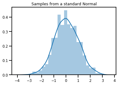
# Plot 1000 samples from a standard normal
samples = normal.sample(1000)
sns.distplot(samples)
plt.title("Samples from a standard Normal")
plt.show()

# Compute the log_prob of a point in the event space of `normal`
normal.log_prob(0.)

<tf.Tensor: shape=(), dtype=float32, numpy=-0.9189385>

# Compute the log_prob of a few points
normal.log_prob([-1., 0., 1.])

<tf.Tensor: shape=(3,), dtype=float32, numpy=array([-1.4189385, -0.9189385, -1.4189385], dtype=float32)>

Distribuciones y formas

Numpy ndarrays y TensorFlow Tensors tienen formas.

TensorFlow de probabilidad Distributions tienen una semántica forma - formas que partición en trozos semánticamente distintas, a pesar de que el mismo trozo de memoria ( Tensor / ndarray ) se utiliza para todo el todo.

• Forma de lotes denota una colección de Distribution s con parámetros distintos
• Forma Evento refiere a la forma de las muestras de la Distribution .

Siempre colocamos formas de lote a la "izquierda" y formas de eventos a la "derecha".

Un lote de escalar-variable Distributions

Los lotes son como distribuciones "vectorizadas": instancias independientes cuyos cálculos ocurren en paralelo.

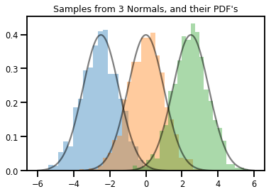
# Create a batch of 3 normals, and plot 1000 samples from each
normals = tfd.Normal([-2.5, 0., 2.5], 1.)  # The scale parameter broadacasts!
print("Batch shape:", normals.batch_shape)
print("Event shape:", normals.event_shape)

Batch shape: (3,)
Event shape: ()

# Samples' shapes go on the left!
samples = normals.sample(1000)
print("Shape of samples:", samples.shape)

Shape of samples: (1000, 3)

# Sample shapes can themselves be more complicated
print("Shape of samples:", normals.sample([10, 10, 10]).shape)

Shape of samples: (10, 10, 10, 3)

# A batch of normals gives a batch of log_probs.
print(normals.log_prob([-2.5, 0., 2.5]))

tf.Tensor([-0.9189385 -0.9189385 -0.9189385], shape=(3,), dtype=float32)

# The computation broadcasts, so a batch of normals applied to a scalar
# also gives a batch of log_probs.
print(normals.log_prob(0.))

tf.Tensor([-4.0439386 -0.9189385 -4.0439386], shape=(3,), dtype=float32)

# Normal numpy-like broadcasting rules apply!
xs = np.linspace(-6, 6, 200)
try:
  normals.log_prob(xs)
except Exception as e:
  print("TFP error:", e.message)

TFP error: Incompatible shapes: [200] vs. [3] [Op:SquaredDifference]

# That fails for the same reason this does:
try:
  np.zeros(200) + np.zeros(3)
except Exception as e:
  print("Numpy error:", e)

Numpy error: operands could not be broadcast together with shapes (200,) (3,)

# But this would work:
a = np.zeros([200, 1]) + np.zeros(3)
print("Broadcast shape:", a.shape)

Broadcast shape: (200, 3)

# And so will this!
xs = np.linspace(-6, 6, 200)[..., np.newaxis]
# => shape = [200, 1]

lps = normals.log_prob(xs)
print("Broadcast log_prob shape:", lps.shape)

Broadcast log_prob shape: (200, 3)

# Summarizing visually
for i in range(3):
  sns.distplot(samples[:, i], kde=False, norm_hist=True)
plt.plot(np.tile(xs, 3), normals.prob(xs), c='k', alpha=.5)
plt.title("Samples from 3 Normals, and their PDF's")
plt.show()

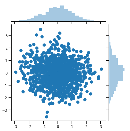
Un vector-variable Distribution

mvn = tfd.MultivariateNormalDiag(loc=[0., 0.], scale_diag = [1., 1.])
print("Batch shape:", mvn.batch_shape)
print("Event shape:", mvn.event_shape)

Batch shape: ()
Event shape: (2,)

samples = mvn.sample(1000)
print("Samples shape:", samples.shape)

Samples shape: (1000, 2)

g = sns.jointplot(samples[:, 0], samples[:, 1], kind='scatter')
plt.show()

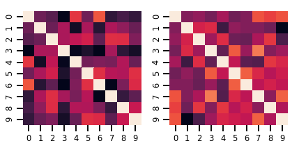
Una matriz-variable Distribution

lkj = tfd.LKJ(dimension=10, concentration=[1.5, 3.0])
print("Batch shape: ", lkj.batch_shape)
print("Event shape: ", lkj.event_shape)

Batch shape:  (2,)
Event shape:  (10, 10)

samples = lkj.sample()
print("Samples shape: ", samples.shape)

Samples shape:  (2, 10, 10)

fig, axes = plt.subplots(nrows=1, ncols=2, figsize=(6, 3))
sns.heatmap(samples[0, ...], ax=axes[0], cbar=False)
sns.heatmap(samples[1, ...], ax=axes[1], cbar=False)
fig.tight_layout()
plt.show()

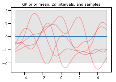
Procesos gaussianos

kernel = tfp.math.psd_kernels.ExponentiatedQuadratic()
xs = np.linspace(-5., 5., 200).reshape([-1, 1])
gp = tfd.GaussianProcess(kernel, index_points=xs)
print("Batch shape:", gp.batch_shape)
print("Event shape:", gp.event_shape)

Batch shape: ()
Event shape: (200,)

upper, lower = gp.mean() + [2 * gp.stddev(), -2 * gp.stddev()]
plt.plot(xs, gp.mean())
plt.fill_between(xs[..., 0], upper, lower, color='k', alpha=.1)
for _ in range(5):
  plt.plot(xs, gp.sample(), c='r', alpha=.3)
plt.title(r"GP prior mean, $2\sigma$ intervals, and samples")
plt.show()

#    *** Bonus question ***
# Why do so many of these functions lie outside the 95% intervals?

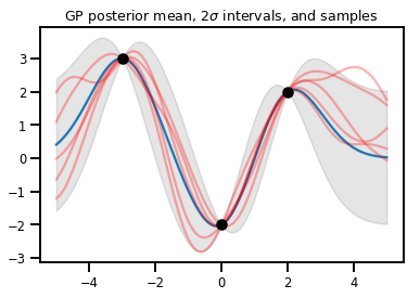
Regresión GP

# Suppose we have some observed data
obs_x = [[-3.], [0.], [2.]]  # Shape 3x1 (3 1-D vectors)
obs_y = [3., -2., 2.]        # Shape 3   (3 scalars)

gprm = tfd.GaussianProcessRegressionModel(kernel, xs, obs_x, obs_y)

upper, lower = gprm.mean() + [2 * gprm.stddev(), -2 * gprm.stddev()]
plt.plot(xs, gprm.mean())
plt.fill_between(xs[..., 0], upper, lower, color='k', alpha=.1)
for _ in range(5):
  plt.plot(xs, gprm.sample(), c='r', alpha=.3)
plt.scatter(obs_x, obs_y, c='k', zorder=3)
plt.title(r"GP posterior mean, $2\sigma$ intervals, and samples")
plt.show()

Biyectores

Los biyectores representan (en su mayoría) funciones suaves e invertibles. Se pueden utilizar para transformar distribuciones, conservando la capacidad de tomar muestras y calcular log_probs. Pueden estar en el tfp.bijectors módulo.

Cada biyector implementa al menos 3 métodos:

• forward ,
• inverse , y
• (al menos) uno de forward_log_det_jacobian y inverse_log_det_jacobian .

¡Con estos ingredientes, podemos transformar una distribución y aún así obtener muestras y registrar problemas del resultado!

En matemáticas, algo descuidadamente

• \(X\) es una variable aleatoria con pdf \(p(x)\)
• \(g\) es una función suave, invertible en el espacio de \(X\)'s
• \(Y = g(X)\) es un nuevo, variable aleatoria transformado
• \(p(Y=y) = p(X=g^{-1}(y)) \cdot |\nabla g^{-1}(y)|\)

Almacenamiento en caché

Los biyectores también almacenan en caché los cálculos directos e inversos y log-det-jacobianos, lo que nos permite ahorrar la repetición de operaciones potencialmente muy costosas.

print_subclasses_from_module(tfp.bijectors, tfp.bijectors.Bijector)

AbsoluteValue, Affine, AffineLinearOperator, AffineScalar, BatchNormalization
Bijector, Blockwise, Chain, CholeskyOuterProduct, CholeskyToInvCholesky
CorrelationCholesky, Cumsum, DiscreteCosineTransform, Exp, Expm1, FFJORD
FillScaleTriL, FillTriangular, FrechetCDF, GeneralizedExtremeValueCDF
GeneralizedPareto, GompertzCDF, GumbelCDF, Identity, Inline, Invert
IteratedSigmoidCentered, KumaraswamyCDF, LambertWTail, Log, Log1p
MaskedAutoregressiveFlow, MatrixInverseTriL, MatvecLU, MoyalCDF, NormalCDF
Ordered, Pad, Permute, PowerTransform, RationalQuadraticSpline, RayleighCDF
RealNVP, Reciprocal, Reshape, Scale, ScaleMatvecDiag, ScaleMatvecLU
ScaleMatvecLinearOperator, ScaleMatvecTriL, ScaleTriL, Shift, ShiftedGompertzCDF
Sigmoid, Sinh, SinhArcsinh, SoftClip, Softfloor, SoftmaxCentered, Softplus
Softsign, Split, Square, Tanh, TransformDiagonal, Transpose, WeibullCDF

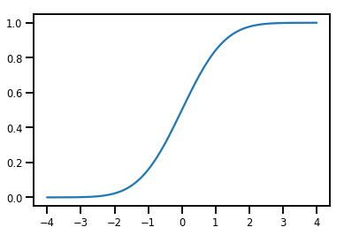
Un simple Bijector

normal_cdf = tfp.bijectors.NormalCDF()
xs = np.linspace(-4., 4., 200)
plt.plot(xs, normal_cdf.forward(xs))
plt.show()

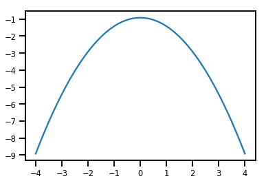
plt.plot(xs, normal_cdf.forward_log_det_jacobian(xs, event_ndims=0))
plt.show()

A Bijector transformar una Distribution

exp_bijector = tfp.bijectors.Exp()
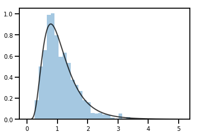
log_normal = exp_bijector(tfd.Normal(0., .5))

samples = log_normal.sample(1000)
xs = np.linspace(1e-10, np.max(samples), 200)
sns.distplot(samples, norm_hist=True, kde=False)
plt.plot(xs, log_normal.prob(xs), c='k', alpha=.75)
plt.show()

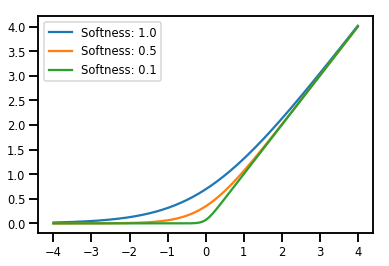
Preparación de lotes Bijectors

# Create a batch of bijectors of shape [3,]
softplus = tfp.bijectors.Softplus(
  hinge_softness=[1., .5, .1])
print("Hinge softness shape:", softplus.hinge_softness.shape)

Hinge softness shape: (3,)

# For broadcasting, we want this to be shape [200, 1]
xs = np.linspace(-4., 4., 200)[..., np.newaxis]
ys = softplus.forward(xs)
print("Forward shape:", ys.shape)

Forward shape: (200, 3)

# Visualization
lines = plt.plot(np.tile(xs, 3), ys)
for line, hs in zip(lines, softplus.hinge_softness):
  line.set_label("Softness: %1.1f" % hs)
plt.legend()
plt.show()

Almacenamiento en caché

# This bijector represents a matrix outer product on the forward pass,
# and a cholesky decomposition on the inverse pass. The latter costs O(N^3)!
bij = tfb.CholeskyOuterProduct()

size = 2500
# Make a big, lower-triangular matrix
big_lower_triangular = tf.eye(size)
# Squaring it gives us a positive-definite matrix
big_positive_definite = bij.forward(big_lower_triangular)

# Caching for the win!
%timeit bij.inverse(big_positive_definite)
%timeit tf.linalg.cholesky(big_positive_definite)

10000 loops, best of 3: 114 µs per loop
1 loops, best of 3: 208 ms per loop

MCMC

TFP ha incorporado soporte para algunos algoritmos estándar de Monte Carlo de la cadena de Markov, incluido el Hamiltonian Monte Carlo.

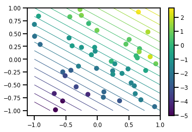
Generar un conjunto de datos

# Generate some data
def f(x, w):
  # Pad x with 1's so we can add bias via matmul
  x = tf.pad(x, [[1, 0], [0, 0]], constant_values=1)
  linop = tf.linalg.LinearOperatorFullMatrix(w[..., np.newaxis])
  result = linop.matmul(x, adjoint=True)
  return result[..., 0, :]

num_features = 2
num_examples = 50
noise_scale = .5
true_w = np.array([-1., 2., 3.])

xs = np.random.uniform(-1., 1., [num_features, num_examples])
ys = f(xs, true_w) + np.random.normal(0., noise_scale, size=num_examples)

# Visualize the data set
plt.scatter(*xs, c=ys, s=100, linewidths=0)

grid = np.meshgrid(*([np.linspace(-1, 1, 100)] * 2))
xs_grid = np.stack(grid, axis=0)
fs_grid = f(xs_grid.reshape([num_features, -1]), true_w)
fs_grid = np.reshape(fs_grid, [100, 100])
plt.colorbar()
plt.contour(xs_grid[0, ...], xs_grid[1, ...], fs_grid, 20, linewidths=1)
plt.show()

Defina nuestra función conjunta log-prob

La posterior no normalizada es el resultado de cierre sobre los datos para formar una aplicación parcial de la prob registro de articulación.

# Define the joint_log_prob function, and our unnormalized posterior.
def joint_log_prob(w, x, y):
  # Our model in maths is
  #   w ~ MVN([0, 0, 0], diag([1, 1, 1]))
  #   y_i ~ Normal(w @ x_i, noise_scale),  i=1..N

  rv_w = tfd.MultivariateNormalDiag(
    loc=np.zeros(num_features + 1),
    scale_diag=np.ones(num_features + 1))

  rv_y = tfd.Normal(f(x, w), noise_scale)
  return (rv_w.log_prob(w) +
          tf.reduce_sum(rv_y.log_prob(y), axis=-1))

# Create our unnormalized target density by currying x and y from the joint.
def unnormalized_posterior(w):
  return joint_log_prob(w, xs, ys)

Compile HMC TransitionKernel y llame a sample_chain

# Create an HMC TransitionKernel
hmc_kernel = tfp.mcmc.HamiltonianMonteCarlo(
  target_log_prob_fn=unnormalized_posterior,
  step_size=np.float64(.1),
  num_leapfrog_steps=2)

# We wrap sample_chain in tf.function, telling TF to precompile a reusable
# computation graph, which will dramatically improve performance.
@tf.function
def run_chain(initial_state, num_results=1000, num_burnin_steps=500):
  return tfp.mcmc.sample_chain(
    num_results=num_results,
    num_burnin_steps=num_burnin_steps,
    current_state=initial_state,
    kernel=hmc_kernel,
    trace_fn=lambda current_state, kernel_results: kernel_results)

initial_state = np.zeros(num_features + 1)
samples, kernel_results = run_chain(initial_state)
print("Acceptance rate:", kernel_results.is_accepted.numpy().mean())

Acceptance rate: 0.915

¡Eso no es genial! Nos gustaría una tasa de aceptación más cercana a .65.

(ver "Escalamiento óptimo para diversos Metropolis-Hastings Algoritmos" , Roberts y Rosenthal, 2001)

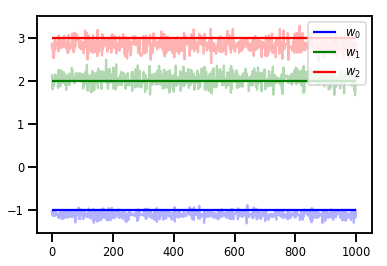
Tamaños de paso adaptables

Podemos concluir nuestra HMC TransitionKernel en un SimpleStepSizeAdaptation "meta-núcleo", que se aplicará alguna lógica (bastante simple heurística) para adaptar el tamaño de paso HMC durante ardiendo. Asignamos el 80% del quemado para adaptar el tamaño del paso y luego dejamos que el 20% restante se vaya solo a mezclar.

# Apply a simple step size adaptation during burnin
@tf.function
def run_chain(initial_state, num_results=1000, num_burnin_steps=500):
  adaptive_kernel = tfp.mcmc.SimpleStepSizeAdaptation(
      hmc_kernel,
      num_adaptation_steps=int(.8 * num_burnin_steps),
      target_accept_prob=np.float64(.65))

  return tfp.mcmc.sample_chain(
    num_results=num_results,
    num_burnin_steps=num_burnin_steps,
    current_state=initial_state,
    kernel=adaptive_kernel,
    trace_fn=lambda cs, kr: kr)

samples, kernel_results = run_chain(
  initial_state=np.zeros(num_features+1))
print("Acceptance rate:", kernel_results.inner_results.is_accepted.numpy().mean())

Acceptance rate: 0.634

# Trace plots
colors = ['b', 'g', 'r']
for i in range(3):
  plt.plot(samples[:, i], c=colors[i], alpha=.3)
  plt.hlines(true_w[i], 0, 1000, zorder=4, color=colors[i], label="$w_{}$".format(i))
plt.legend(loc='upper right')
plt.show()

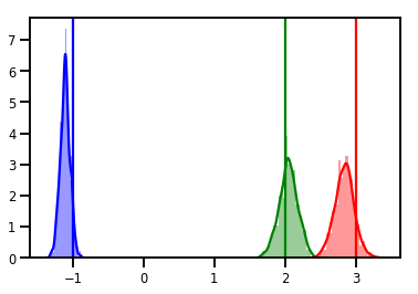
# Histogram of samples
for i in range(3):
  sns.distplot(samples[:, i], color=colors[i])
ymax = plt.ylim()[1]
for i in range(3):
  plt.vlines(true_w[i], 0, ymax, color=colors[i])
plt.ylim(0, ymax)
plt.show()

Diagnóstico

Los diagramas de seguimiento son agradables, ¡pero los diagnósticos son mejores!

Primero necesitamos ejecutar múltiples cadenas. Esto es tan simple como darle un lote de initial_state tensores.

# Instead of a single set of initial w's, we create a batch of 8.
num_chains = 8
initial_state = np.zeros([num_chains, num_features + 1])

chains, kernel_results = run_chain(initial_state)

r_hat = tfp.mcmc.potential_scale_reduction(chains)
print("Acceptance rate:", kernel_results.inner_results.is_accepted.numpy().mean())
print("R-hat diagnostic (per latent variable):", r_hat.numpy())

Acceptance rate: 0.59175
R-hat diagnostic (per latent variable): [0.99998395 0.99932185 0.9997064 ]

Muestreo de la escala de ruido

# Define the joint_log_prob function, and our unnormalized posterior.
def joint_log_prob(w, sigma, x, y):
  # Our model in maths is
  #   w ~ MVN([0, 0, 0], diag([1, 1, 1]))
  #   y_i ~ Normal(w @ x_i, noise_scale),  i=1..N

  rv_w = tfd.MultivariateNormalDiag(
    loc=np.zeros(num_features + 1),
    scale_diag=np.ones(num_features + 1))

  rv_sigma = tfd.LogNormal(np.float64(1.), np.float64(5.))

  rv_y = tfd.Normal(f(x, w), sigma[..., np.newaxis])
  return (rv_w.log_prob(w) +
          rv_sigma.log_prob(sigma) +
          tf.reduce_sum(rv_y.log_prob(y), axis=-1))

# Create our unnormalized target density by currying x and y from the joint.
def unnormalized_posterior(w, sigma):
  return joint_log_prob(w, sigma, xs, ys)


# Create an HMC TransitionKernel
hmc_kernel = tfp.mcmc.HamiltonianMonteCarlo(
  target_log_prob_fn=unnormalized_posterior,
  step_size=np.float64(.1),
  num_leapfrog_steps=4)



# Create a TransformedTransitionKernl
transformed_kernel = tfp.mcmc.TransformedTransitionKernel(
    inner_kernel=hmc_kernel,
    bijector=[tfb.Identity(),    # w
              tfb.Invert(tfb.Softplus())])   # sigma


# Apply a simple step size adaptation during burnin
@tf.function
def run_chain(initial_state, num_results=1000, num_burnin_steps=500):
  adaptive_kernel = tfp.mcmc.SimpleStepSizeAdaptation(
      transformed_kernel,
      num_adaptation_steps=int(.8 * num_burnin_steps),
      target_accept_prob=np.float64(.75))

  return tfp.mcmc.sample_chain(
    num_results=num_results,
    num_burnin_steps=num_burnin_steps,
    current_state=initial_state,
    kernel=adaptive_kernel,
    seed=(0, 1),
    trace_fn=lambda cs, kr: kr)


# Instead of a single set of initial w's, we create a batch of 8.
num_chains = 8
initial_state = [np.zeros([num_chains, num_features + 1]),
                 .54 * np.ones([num_chains], dtype=np.float64)]

chains, kernel_results = run_chain(initial_state)

r_hat = tfp.mcmc.potential_scale_reduction(chains)
print("Acceptance rate:", kernel_results.inner_results.inner_results.is_accepted.numpy().mean())
print("R-hat diagnostic (per w variable):", r_hat[0].numpy())
print("R-hat diagnostic (sigma):", r_hat[1].numpy())

Acceptance rate: 0.715875
R-hat diagnostic (per w variable): [1.0000073  1.00458208 1.00450512]
R-hat diagnostic (sigma): 1.0092056996149859

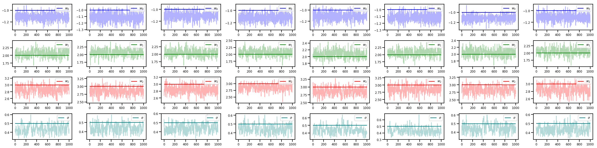
w_chains, sigma_chains = chains

# Trace plots of w (one of 8 chains)
colors = ['b', 'g', 'r', 'teal']
fig, axes = plt.subplots(4, num_chains, figsize=(4 * num_chains, 8))
for j in range(num_chains):
  for i in range(3):
    ax = axes[i][j]
    ax.plot(w_chains[:, j, i], c=colors[i], alpha=.3)
    ax.hlines(true_w[i], 0, 1000, zorder=4, color=colors[i], label="$w_{}$".format(i))
    ax.legend(loc='upper right')
  ax = axes[3][j]
  ax.plot(sigma_chains[:, j], alpha=.3, c=colors[3])
  ax.hlines(noise_scale, 0, 1000, zorder=4, color=colors[3], label=r"$\sigma$".format(i))
  ax.legend(loc='upper right')
fig.tight_layout()
plt.show()

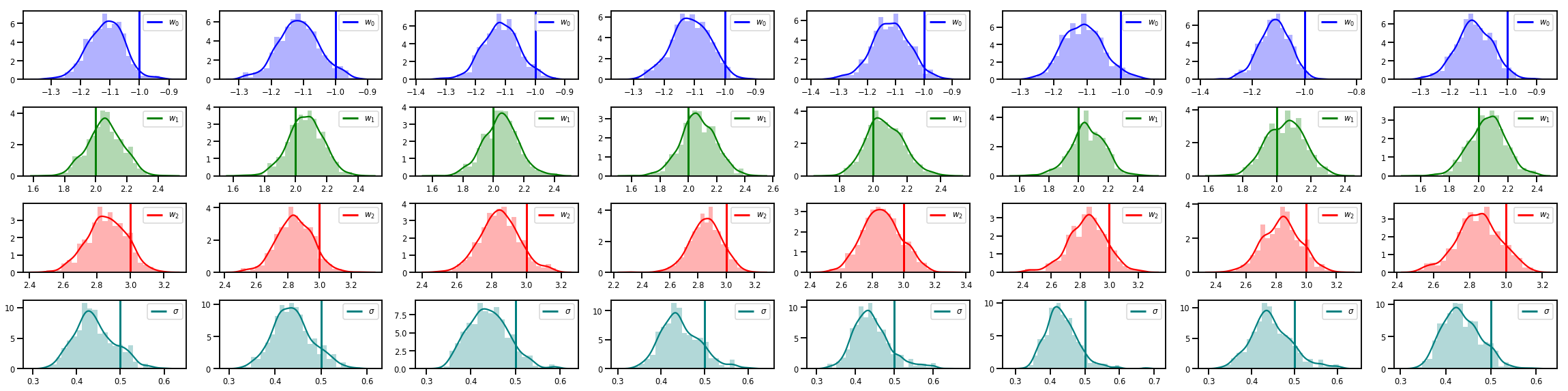
# Histogram of samples of w
fig, axes = plt.subplots(4, num_chains, figsize=(4 * num_chains, 8))
for j in range(num_chains):
  for i in range(3):
    ax = axes[i][j]
    sns.distplot(w_chains[:, j, i], color=colors[i], norm_hist=True, ax=ax, hist_kws={'alpha': .3})
  for i in range(3):
    ax = axes[i][j]
    ymax = ax.get_ylim()[1]
    ax.vlines(true_w[i], 0, ymax, color=colors[i], label="$w_{}$".format(i), linewidth=3)
    ax.set_ylim(0, ymax)
    ax.legend(loc='upper right')


  ax = axes[3][j]
  sns.distplot(sigma_chains[:, j], color=colors[3], norm_hist=True, ax=ax, hist_kws={'alpha': .3})
  ymax = ax.get_ylim()[1]
  ax.vlines(noise_scale, 0, ymax, color=colors[3], label=r"$\sigma$".format(i), linewidth=3)
  ax.set_ylim(0, ymax)
  ax.legend(loc='upper right')
fig.tight_layout()
plt.show()

¡Hay mucho más!

Echa un vistazo a estas interesantes publicaciones de blog y ejemplos:

• Estructural de series temporales de apoyo del blog colab
• Capas probabilístico Keras (entrada: Tensor, salida: Distribución!) El blog colab
  • Otro ejemplo Capas: VAE el blog colab
• Gaussian proceso de regresión colab y variable latente Modelado colab

Más ejemplos y cuadernos en nuestra GitHub aquí !