Visite guidée de la probabilité TensorFlow

Voir sur TensorFlow.org

Exécuter dans Google Colab

Voir la source sur GitHub

Télécharger le cahier

Dans ce Colab, nous explorons certaines des fonctionnalités fondamentales de TensorFlow Probability.

Dépendances et prérequis

Importer

from pprint import pprint
import matplotlib.pyplot as plt
import numpy as np
import seaborn as sns

import tensorflow.compat.v2 as tf
tf.enable_v2_behavior()

import tensorflow_probability as tfp

sns.reset_defaults()
sns.set_context(context='talk',font_scale=0.7)
plt.rcParams['image.cmap'] = 'viridis'

%matplotlib inline

tfd = tfp.distributions
tfb = tfp.bijectors

Utilitaires

def print_subclasses_from_module(module, base_class, maxwidth=80):
  import functools, inspect, sys
  subclasses = [name for name, obj in inspect.getmembers(module)
                if inspect.isclass(obj) and issubclass(obj, base_class)]
  def red(acc, x):
    if not acc or len(acc[-1]) + len(x) + 2 > maxwidth:
      acc.append(x)
    else:
      acc[-1] += ", " + x
    return acc
  print('\n'.join(functools.reduce(red, subclasses, [])))

Présenter

• TensorFlow
• Probabilité TensorFlow
  • Répartition
  • Bijecteurs
  • MCMC
  • ...et plus!

Préambule : TensorFlow

TensorFlow est une bibliothèque de calcul scientifique.

Elle supporte

• beaucoup d'opérations mathématiques
• calcul vectorisé efficace
• accélération matérielle facile
• différenciation automatique

Vectorisation

• La vectorisation accélère les choses !
• Cela signifie aussi que nous pensons beaucoup aux formes

mats = tf.random.uniform(shape=[1000, 10, 10])
vecs = tf.random.uniform(shape=[1000, 10, 1])

def for_loop_solve():
  return np.array(
    [tf.linalg.solve(mats[i, ...], vecs[i, ...]) for i in range(1000)])

def vectorized_solve():
  return tf.linalg.solve(mats, vecs)

# Vectorization for the win!
%timeit for_loop_solve()
%timeit vectorized_solve()

1 loops, best of 3: 2 s per loop
1000 loops, best of 3: 653 µs per loop

Accélération matérielle

# Code can run seamlessly on a GPU, just change Colab runtime type
# in the 'Runtime' menu.
if tf.test.gpu_device_name() == '/device:GPU:0':
  print("Using a GPU")
else:
  print("Using a CPU")

Using a CPU

Différenciation automatique

a = tf.constant(np.pi)
b = tf.constant(np.e)
with tf.GradientTape() as tape:
  tape.watch([a, b])
  c = .5 * (a**2 + b**2)
grads = tape.gradient(c, [a, b])
print(grads[0])
print(grads[1])

tf.Tensor(3.1415927, shape=(), dtype=float32)
tf.Tensor(2.7182817, shape=(), dtype=float32)

Probabilité TensorFlow

TensorFlow Probability est une bibliothèque pour le raisonnement probabiliste et l'analyse statistique dans TensorFlow.

Nous sommes favorables à la modélisation, l' inférence, et critique à travers la composition de composants modulaires de bas niveau.

Blocs de construction de bas niveau

• Répartition
• Bijecteurs

Constructions de (plus) niveau élevé

• Chaîne de Markov Monte Carlo
• Couches probabilistes
• Séries temporelles structurelles
• Modèles linéaires généralisés
• Optimiseurs

Répartition

Un tfp.distributions.Distribution est une classe avec deux méthodes principales: sample et log_prob .

TFP a beaucoup de distributions !

print_subclasses_from_module(tfp.distributions, tfp.distributions.Distribution)

Autoregressive, BatchReshape, Bates, Bernoulli, Beta, BetaBinomial, Binomial
Blockwise, Categorical, Cauchy, Chi, Chi2, CholeskyLKJ, ContinuousBernoulli
Deterministic, Dirichlet, DirichletMultinomial, Distribution, DoublesidedMaxwell
Empirical, ExpGamma, ExpRelaxedOneHotCategorical, Exponential, FiniteDiscrete
Gamma, GammaGamma, GaussianProcess, GaussianProcessRegressionModel
GeneralizedNormal, GeneralizedPareto, Geometric, Gumbel, HalfCauchy, HalfNormal
HalfStudentT, HiddenMarkovModel, Horseshoe, Independent, InverseGamma
InverseGaussian, JohnsonSU, JointDistribution, JointDistributionCoroutine
JointDistributionCoroutineAutoBatched, JointDistributionNamed
JointDistributionNamedAutoBatched, JointDistributionSequential
JointDistributionSequentialAutoBatched, Kumaraswamy, LKJ, Laplace
LinearGaussianStateSpaceModel, LogLogistic, LogNormal, Logistic, LogitNormal
Mixture, MixtureSameFamily, Moyal, Multinomial, MultivariateNormalDiag
MultivariateNormalDiagPlusLowRank, MultivariateNormalFullCovariance
MultivariateNormalLinearOperator, MultivariateNormalTriL
MultivariateStudentTLinearOperator, NegativeBinomial, Normal, OneHotCategorical
OrderedLogistic, PERT, Pareto, PixelCNN, PlackettLuce, Poisson
PoissonLogNormalQuadratureCompound, PowerSpherical, ProbitBernoulli
QuantizedDistribution, RelaxedBernoulli, RelaxedOneHotCategorical, Sample
SinhArcsinh, SphericalUniform, StudentT, StudentTProcess
TransformedDistribution, Triangular, TruncatedCauchy, TruncatedNormal, Uniform
VariationalGaussianProcess, VectorDeterministic, VonMises
VonMisesFisher, Weibull, WishartLinearOperator, WishartTriL, Zipf

Un simple scalaire variate Distribution

# A standard normal
normal = tfd.Normal(loc=0., scale=1.)
print(normal)

tfp.distributions.Normal("Normal", batch_shape=[], event_shape=[], dtype=float32)

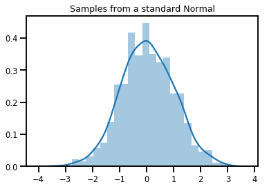
# Plot 1000 samples from a standard normal
samples = normal.sample(1000)
sns.distplot(samples)
plt.title("Samples from a standard Normal")
plt.show()

# Compute the log_prob of a point in the event space of `normal`
normal.log_prob(0.)

<tf.Tensor: shape=(), dtype=float32, numpy=-0.9189385>

# Compute the log_prob of a few points
normal.log_prob([-1., 0., 1.])

<tf.Tensor: shape=(3,), dtype=float32, numpy=array([-1.4189385, -0.9189385, -1.4189385], dtype=float32)>

Distributions et formes

Numpy ndarrays et tensorflow Tensors ont des formes.

Tensorflow Probabilité Les Distributions ont une sémantique de forme - formes de séparation , nous en morceaux sémantiquement distinctes, même si le même morceau de mémoire ( Tensor / ndarray ) est utilisé pour tout l' ensemble.

• Forme de lot désigne un ensemble de Distribution s avec des paramètres distincts
• Forme de l' événement indique la forme d'échantillons de la Distribution .

Nous mettons toujours des formes de lots à « gauche » et des formes d'événements à « droite ».

Un lot de scalaire variate Distributions

Les lots sont comme des distributions « vectorisées » : des instances indépendantes dont les calculs se font en parallèle.

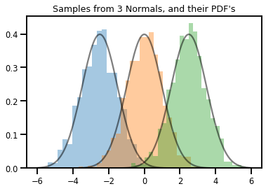
# Create a batch of 3 normals, and plot 1000 samples from each
normals = tfd.Normal([-2.5, 0., 2.5], 1.)  # The scale parameter broadacasts!
print("Batch shape:", normals.batch_shape)
print("Event shape:", normals.event_shape)

Batch shape: (3,)
Event shape: ()

# Samples' shapes go on the left!
samples = normals.sample(1000)
print("Shape of samples:", samples.shape)

Shape of samples: (1000, 3)

# Sample shapes can themselves be more complicated
print("Shape of samples:", normals.sample([10, 10, 10]).shape)

Shape of samples: (10, 10, 10, 3)

# A batch of normals gives a batch of log_probs.
print(normals.log_prob([-2.5, 0., 2.5]))

tf.Tensor([-0.9189385 -0.9189385 -0.9189385], shape=(3,), dtype=float32)

# The computation broadcasts, so a batch of normals applied to a scalar
# also gives a batch of log_probs.
print(normals.log_prob(0.))

tf.Tensor([-4.0439386 -0.9189385 -4.0439386], shape=(3,), dtype=float32)

# Normal numpy-like broadcasting rules apply!
xs = np.linspace(-6, 6, 200)
try:
  normals.log_prob(xs)
except Exception as e:
  print("TFP error:", e.message)

TFP error: Incompatible shapes: [200] vs. [3] [Op:SquaredDifference]

# That fails for the same reason this does:
try:
  np.zeros(200) + np.zeros(3)
except Exception as e:
  print("Numpy error:", e)

Numpy error: operands could not be broadcast together with shapes (200,) (3,)

# But this would work:
a = np.zeros([200, 1]) + np.zeros(3)
print("Broadcast shape:", a.shape)

Broadcast shape: (200, 3)

# And so will this!
xs = np.linspace(-6, 6, 200)[..., np.newaxis]
# => shape = [200, 1]

lps = normals.log_prob(xs)
print("Broadcast log_prob shape:", lps.shape)

Broadcast log_prob shape: (200, 3)

# Summarizing visually
for i in range(3):
  sns.distplot(samples[:, i], kde=False, norm_hist=True)
plt.plot(np.tile(xs, 3), normals.prob(xs), c='k', alpha=.5)
plt.title("Samples from 3 Normals, and their PDF's")
plt.show()

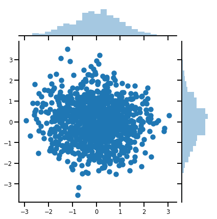
Un vecteur-variate Distribution

mvn = tfd.MultivariateNormalDiag(loc=[0., 0.], scale_diag = [1., 1.])
print("Batch shape:", mvn.batch_shape)
print("Event shape:", mvn.event_shape)

Batch shape: ()
Event shape: (2,)

samples = mvn.sample(1000)
print("Samples shape:", samples.shape)

Samples shape: (1000, 2)

g = sns.jointplot(samples[:, 0], samples[:, 1], kind='scatter')
plt.show()

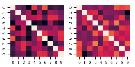
Une matrice-variate Distribution

lkj = tfd.LKJ(dimension=10, concentration=[1.5, 3.0])
print("Batch shape: ", lkj.batch_shape)
print("Event shape: ", lkj.event_shape)

Batch shape:  (2,)
Event shape:  (10, 10)

samples = lkj.sample()
print("Samples shape: ", samples.shape)

Samples shape:  (2, 10, 10)

fig, axes = plt.subplots(nrows=1, ncols=2, figsize=(6, 3))
sns.heatmap(samples[0, ...], ax=axes[0], cbar=False)
sns.heatmap(samples[1, ...], ax=axes[1], cbar=False)
fig.tight_layout()
plt.show()

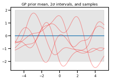
Processus gaussiens

kernel = tfp.math.psd_kernels.ExponentiatedQuadratic()
xs = np.linspace(-5., 5., 200).reshape([-1, 1])
gp = tfd.GaussianProcess(kernel, index_points=xs)
print("Batch shape:", gp.batch_shape)
print("Event shape:", gp.event_shape)

Batch shape: ()
Event shape: (200,)

upper, lower = gp.mean() + [2 * gp.stddev(), -2 * gp.stddev()]
plt.plot(xs, gp.mean())
plt.fill_between(xs[..., 0], upper, lower, color='k', alpha=.1)
for _ in range(5):
  plt.plot(xs, gp.sample(), c='r', alpha=.3)
plt.title(r"GP prior mean, $2\sigma$ intervals, and samples")
plt.show()

#    *** Bonus question ***
# Why do so many of these functions lie outside the 95% intervals?

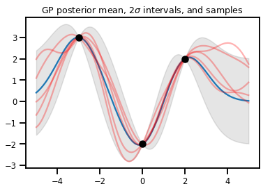
Régression GP

# Suppose we have some observed data
obs_x = [[-3.], [0.], [2.]]  # Shape 3x1 (3 1-D vectors)
obs_y = [3., -2., 2.]        # Shape 3   (3 scalars)

gprm = tfd.GaussianProcessRegressionModel(kernel, xs, obs_x, obs_y)

upper, lower = gprm.mean() + [2 * gprm.stddev(), -2 * gprm.stddev()]
plt.plot(xs, gprm.mean())
plt.fill_between(xs[..., 0], upper, lower, color='k', alpha=.1)
for _ in range(5):
  plt.plot(xs, gprm.sample(), c='r', alpha=.3)
plt.scatter(obs_x, obs_y, c='k', zorder=3)
plt.title(r"GP posterior mean, $2\sigma$ intervals, and samples")
plt.show()

Bijecteurs

Les bijecteurs représentent (principalement) des fonctions lisses et inversibles. Ils peuvent être utilisés pour transformer des distributions, en préservant la possibilité de prélever des échantillons et de calculer log_probs. Ils peuvent être dans le tfp.bijectors module.

Chaque bijecteur implémente au moins 3 méthodes :

• forward ,
• inverse , et
• (au moins) une des forward_log_det_jacobian et inverse_log_det_jacobian .

Avec ces ingrédients, nous pouvons transformer une distribution tout en obtenant des échantillons et en enregistrant des problèmes à partir du résultat !

En maths, un peu négligemment

• \(X\) est une variable aléatoire pdf \(p(x)\)
• \(g\) est une fonction lisse, inversible sur l'espace des \(X\)« s
• \(Y = g(X)\) est une nouvelle, transformée variable aléatoire
• \(p(Y=y) = p(X=g^{-1}(y)) \cdot |\nabla g^{-1}(y)|\)

Mise en cache

Les bijecteurs mettent également en cache les calculs directs et inverses, et les log-det-Jacobians, ce qui nous permet d'éviter de répéter des opérations potentiellement très coûteuses !

print_subclasses_from_module(tfp.bijectors, tfp.bijectors.Bijector)

AbsoluteValue, Affine, AffineLinearOperator, AffineScalar, BatchNormalization
Bijector, Blockwise, Chain, CholeskyOuterProduct, CholeskyToInvCholesky
CorrelationCholesky, Cumsum, DiscreteCosineTransform, Exp, Expm1, FFJORD
FillScaleTriL, FillTriangular, FrechetCDF, GeneralizedExtremeValueCDF
GeneralizedPareto, GompertzCDF, GumbelCDF, Identity, Inline, Invert
IteratedSigmoidCentered, KumaraswamyCDF, LambertWTail, Log, Log1p
MaskedAutoregressiveFlow, MatrixInverseTriL, MatvecLU, MoyalCDF, NormalCDF
Ordered, Pad, Permute, PowerTransform, RationalQuadraticSpline, RayleighCDF
RealNVP, Reciprocal, Reshape, Scale, ScaleMatvecDiag, ScaleMatvecLU
ScaleMatvecLinearOperator, ScaleMatvecTriL, ScaleTriL, Shift, ShiftedGompertzCDF
Sigmoid, Sinh, SinhArcsinh, SoftClip, Softfloor, SoftmaxCentered, Softplus
Softsign, Split, Square, Tanh, TransformDiagonal, Transpose, WeibullCDF

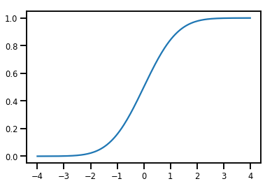
Un simple Bijector

normal_cdf = tfp.bijectors.NormalCDF()
xs = np.linspace(-4., 4., 200)
plt.plot(xs, normal_cdf.forward(xs))
plt.show()

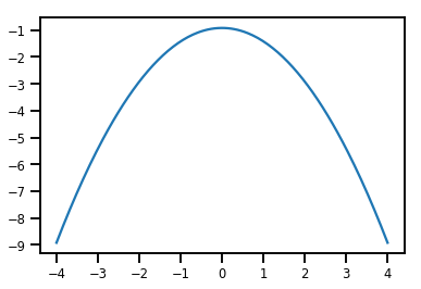
plt.plot(xs, normal_cdf.forward_log_det_jacobian(xs, event_ndims=0))
plt.show()

A Bijector transformation d' une Distribution

exp_bijector = tfp.bijectors.Exp()
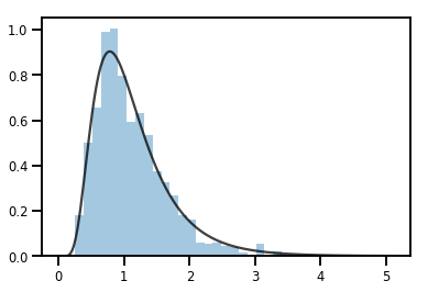
log_normal = exp_bijector(tfd.Normal(0., .5))

samples = log_normal.sample(1000)
xs = np.linspace(1e-10, np.max(samples), 200)
sns.distplot(samples, norm_hist=True, kde=False)
plt.plot(xs, log_normal.prob(xs), c='k', alpha=.75)
plt.show()

batching Bijectors

# Create a batch of bijectors of shape [3,]
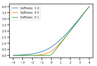
softplus = tfp.bijectors.Softplus(
  hinge_softness=[1., .5, .1])
print("Hinge softness shape:", softplus.hinge_softness.shape)

Hinge softness shape: (3,)

# For broadcasting, we want this to be shape [200, 1]
xs = np.linspace(-4., 4., 200)[..., np.newaxis]
ys = softplus.forward(xs)
print("Forward shape:", ys.shape)

Forward shape: (200, 3)

# Visualization
lines = plt.plot(np.tile(xs, 3), ys)
for line, hs in zip(lines, softplus.hinge_softness):
  line.set_label("Softness: %1.1f" % hs)
plt.legend()
plt.show()

Mise en cache

# This bijector represents a matrix outer product on the forward pass,
# and a cholesky decomposition on the inverse pass. The latter costs O(N^3)!
bij = tfb.CholeskyOuterProduct()

size = 2500
# Make a big, lower-triangular matrix
big_lower_triangular = tf.eye(size)
# Squaring it gives us a positive-definite matrix
big_positive_definite = bij.forward(big_lower_triangular)

# Caching for the win!
%timeit bij.inverse(big_positive_definite)
%timeit tf.linalg.cholesky(big_positive_definite)

10000 loops, best of 3: 114 µs per loop
1 loops, best of 3: 208 ms per loop

MCMC

TFP a intégré la prise en charge de certains algorithmes de Monte Carlo à chaîne de Markov standard, notamment le Monte Carlo hamiltonien.

Générer un ensemble de données

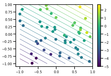
# Generate some data
def f(x, w):
  # Pad x with 1's so we can add bias via matmul
  x = tf.pad(x, [[1, 0], [0, 0]], constant_values=1)
  linop = tf.linalg.LinearOperatorFullMatrix(w[..., np.newaxis])
  result = linop.matmul(x, adjoint=True)
  return result[..., 0, :]

num_features = 2
num_examples = 50
noise_scale = .5
true_w = np.array([-1., 2., 3.])

xs = np.random.uniform(-1., 1., [num_features, num_examples])
ys = f(xs, true_w) + np.random.normal(0., noise_scale, size=num_examples)

# Visualize the data set
plt.scatter(*xs, c=ys, s=100, linewidths=0)

grid = np.meshgrid(*([np.linspace(-1, 1, 100)] * 2))
xs_grid = np.stack(grid, axis=0)
fs_grid = f(xs_grid.reshape([num_features, -1]), true_w)
fs_grid = np.reshape(fs_grid, [100, 100])
plt.colorbar()
plt.contour(xs_grid[0, ...], xs_grid[1, ...], fs_grid, 20, linewidths=1)
plt.show()

Définir notre fonction jointe log-prob

Le postérieur non normalisé est le résultat de la fermeture sur les données pour former une application partielle de l'prob journal commun.

# Define the joint_log_prob function, and our unnormalized posterior.
def joint_log_prob(w, x, y):
  # Our model in maths is
  #   w ~ MVN([0, 0, 0], diag([1, 1, 1]))
  #   y_i ~ Normal(w @ x_i, noise_scale),  i=1..N

  rv_w = tfd.MultivariateNormalDiag(
    loc=np.zeros(num_features + 1),
    scale_diag=np.ones(num_features + 1))

  rv_y = tfd.Normal(f(x, w), noise_scale)
  return (rv_w.log_prob(w) +
          tf.reduce_sum(rv_y.log_prob(y), axis=-1))

# Create our unnormalized target density by currying x and y from the joint.
def unnormalized_posterior(w):
  return joint_log_prob(w, xs, ys)

Générez HMC TransitionKernel et appelez sample_chain

# Create an HMC TransitionKernel
hmc_kernel = tfp.mcmc.HamiltonianMonteCarlo(
  target_log_prob_fn=unnormalized_posterior,
  step_size=np.float64(.1),
  num_leapfrog_steps=2)

# We wrap sample_chain in tf.function, telling TF to precompile a reusable
# computation graph, which will dramatically improve performance.
@tf.function
def run_chain(initial_state, num_results=1000, num_burnin_steps=500):
  return tfp.mcmc.sample_chain(
    num_results=num_results,
    num_burnin_steps=num_burnin_steps,
    current_state=initial_state,
    kernel=hmc_kernel,
    trace_fn=lambda current_state, kernel_results: kernel_results)

initial_state = np.zeros(num_features + 1)
samples, kernel_results = run_chain(initial_state)
print("Acceptance rate:", kernel_results.is_accepted.numpy().mean())

Acceptance rate: 0.915

C'est pas génial ! Nous aimerions un taux d'acceptation plus proche de 0,65.

(voir "Mise à l' échelle optimale pour divers algorithmes Metropolis-Hastings" , Roberts & Rosenthal, 2001)

Tailles de pas adaptatives

Nous pouvons envelopper notre HMC TransitionKernel dans une SimpleStepSizeAdaptation « méta-noyau », qui applique une logique (plutôt simple heuristique) pour adapter la taille de l' étape de la console HMC au cours Burnin. Nous attribuons 80 % de burnin pour adapter la taille des étapes, puis laissons les 20 % restants uniquement au mélange.

# Apply a simple step size adaptation during burnin
@tf.function
def run_chain(initial_state, num_results=1000, num_burnin_steps=500):
  adaptive_kernel = tfp.mcmc.SimpleStepSizeAdaptation(
      hmc_kernel,
      num_adaptation_steps=int(.8 * num_burnin_steps),
      target_accept_prob=np.float64(.65))

  return tfp.mcmc.sample_chain(
    num_results=num_results,
    num_burnin_steps=num_burnin_steps,
    current_state=initial_state,
    kernel=adaptive_kernel,
    trace_fn=lambda cs, kr: kr)

samples, kernel_results = run_chain(
  initial_state=np.zeros(num_features+1))
print("Acceptance rate:", kernel_results.inner_results.is_accepted.numpy().mean())

Acceptance rate: 0.634

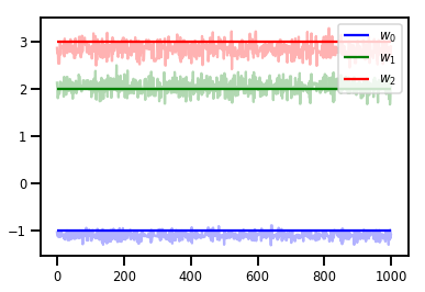
# Trace plots
colors = ['b', 'g', 'r']
for i in range(3):
  plt.plot(samples[:, i], c=colors[i], alpha=.3)
  plt.hlines(true_w[i], 0, 1000, zorder=4, color=colors[i], label="$w_{}$".format(i))
plt.legend(loc='upper right')
plt.show()

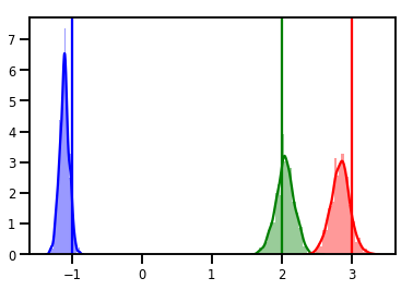
# Histogram of samples
for i in range(3):
  sns.distplot(samples[:, i], color=colors[i])
ymax = plt.ylim()[1]
for i in range(3):
  plt.vlines(true_w[i], 0, ymax, color=colors[i])
plt.ylim(0, ymax)
plt.show()

Diagnostique

Les tracés de trace sont sympas, mais les diagnostics sont plus agréables !

Nous devons d'abord exécuter plusieurs chaînes. Ceci est aussi simple que de donner un lot de initial_state tenseurs.

# Instead of a single set of initial w's, we create a batch of 8.
num_chains = 8
initial_state = np.zeros([num_chains, num_features + 1])

chains, kernel_results = run_chain(initial_state)

r_hat = tfp.mcmc.potential_scale_reduction(chains)
print("Acceptance rate:", kernel_results.inner_results.is_accepted.numpy().mean())
print("R-hat diagnostic (per latent variable):", r_hat.numpy())

Acceptance rate: 0.59175
R-hat diagnostic (per latent variable): [0.99998395 0.99932185 0.9997064 ]

Échantillonnage de l'échelle de bruit

# Define the joint_log_prob function, and our unnormalized posterior.
def joint_log_prob(w, sigma, x, y):
  # Our model in maths is
  #   w ~ MVN([0, 0, 0], diag([1, 1, 1]))
  #   y_i ~ Normal(w @ x_i, noise_scale),  i=1..N

  rv_w = tfd.MultivariateNormalDiag(
    loc=np.zeros(num_features + 1),
    scale_diag=np.ones(num_features + 1))

  rv_sigma = tfd.LogNormal(np.float64(1.), np.float64(5.))

  rv_y = tfd.Normal(f(x, w), sigma[..., np.newaxis])
  return (rv_w.log_prob(w) +
          rv_sigma.log_prob(sigma) +
          tf.reduce_sum(rv_y.log_prob(y), axis=-1))

# Create our unnormalized target density by currying x and y from the joint.
def unnormalized_posterior(w, sigma):
  return joint_log_prob(w, sigma, xs, ys)


# Create an HMC TransitionKernel
hmc_kernel = tfp.mcmc.HamiltonianMonteCarlo(
  target_log_prob_fn=unnormalized_posterior,
  step_size=np.float64(.1),
  num_leapfrog_steps=4)



# Create a TransformedTransitionKernl
transformed_kernel = tfp.mcmc.TransformedTransitionKernel(
    inner_kernel=hmc_kernel,
    bijector=[tfb.Identity(),    # w
              tfb.Invert(tfb.Softplus())])   # sigma


# Apply a simple step size adaptation during burnin
@tf.function
def run_chain(initial_state, num_results=1000, num_burnin_steps=500):
  adaptive_kernel = tfp.mcmc.SimpleStepSizeAdaptation(
      transformed_kernel,
      num_adaptation_steps=int(.8 * num_burnin_steps),
      target_accept_prob=np.float64(.75))

  return tfp.mcmc.sample_chain(
    num_results=num_results,
    num_burnin_steps=num_burnin_steps,
    current_state=initial_state,
    kernel=adaptive_kernel,
    seed=(0, 1),
    trace_fn=lambda cs, kr: kr)


# Instead of a single set of initial w's, we create a batch of 8.
num_chains = 8
initial_state = [np.zeros([num_chains, num_features + 1]),
                 .54 * np.ones([num_chains], dtype=np.float64)]

chains, kernel_results = run_chain(initial_state)

r_hat = tfp.mcmc.potential_scale_reduction(chains)
print("Acceptance rate:", kernel_results.inner_results.inner_results.is_accepted.numpy().mean())
print("R-hat diagnostic (per w variable):", r_hat[0].numpy())
print("R-hat diagnostic (sigma):", r_hat[1].numpy())

Acceptance rate: 0.715875
R-hat diagnostic (per w variable): [1.0000073  1.00458208 1.00450512]
R-hat diagnostic (sigma): 1.0092056996149859

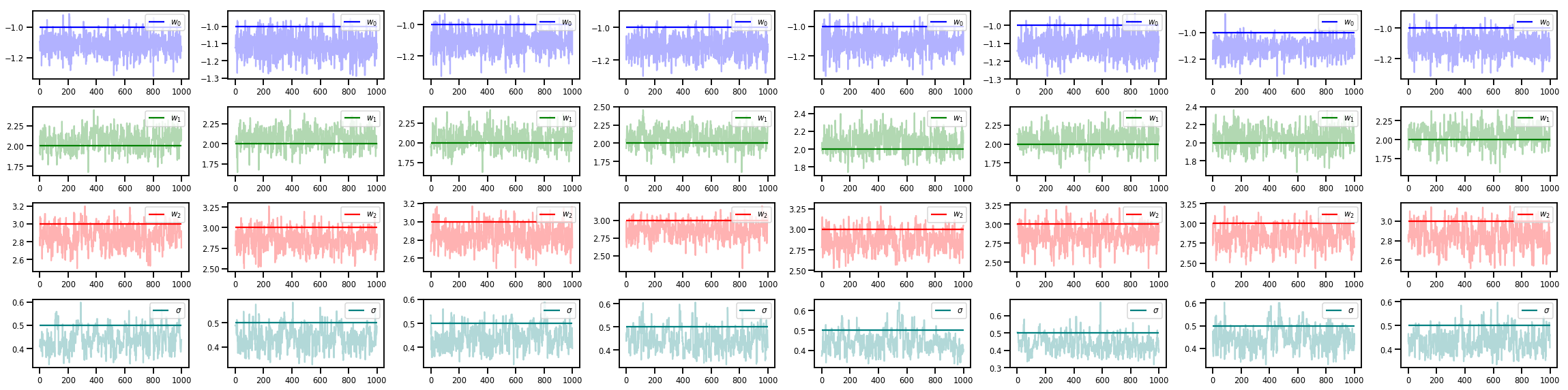
w_chains, sigma_chains = chains

# Trace plots of w (one of 8 chains)
colors = ['b', 'g', 'r', 'teal']
fig, axes = plt.subplots(4, num_chains, figsize=(4 * num_chains, 8))
for j in range(num_chains):
  for i in range(3):
    ax = axes[i][j]
    ax.plot(w_chains[:, j, i], c=colors[i], alpha=.3)
    ax.hlines(true_w[i], 0, 1000, zorder=4, color=colors[i], label="$w_{}$".format(i))
    ax.legend(loc='upper right')
  ax = axes[3][j]
  ax.plot(sigma_chains[:, j], alpha=.3, c=colors[3])
  ax.hlines(noise_scale, 0, 1000, zorder=4, color=colors[3], label=r"$\sigma$".format(i))
  ax.legend(loc='upper right')
fig.tight_layout()
plt.show()

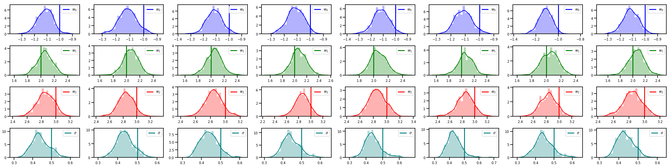
# Histogram of samples of w
fig, axes = plt.subplots(4, num_chains, figsize=(4 * num_chains, 8))
for j in range(num_chains):
  for i in range(3):
    ax = axes[i][j]
    sns.distplot(w_chains[:, j, i], color=colors[i], norm_hist=True, ax=ax, hist_kws={'alpha': .3})
  for i in range(3):
    ax = axes[i][j]
    ymax = ax.get_ylim()[1]
    ax.vlines(true_w[i], 0, ymax, color=colors[i], label="$w_{}$".format(i), linewidth=3)
    ax.set_ylim(0, ymax)
    ax.legend(loc='upper right')


  ax = axes[3][j]
  sns.distplot(sigma_chains[:, j], color=colors[3], norm_hist=True, ax=ax, hist_kws={'alpha': .3})
  ymax = ax.get_ylim()[1]
  ax.vlines(noise_scale, 0, ymax, color=colors[3], label=r"$\sigma$".format(i), linewidth=3)
  ax.set_ylim(0, ymax)
  ax.legend(loc='upper right')
fig.tight_layout()
plt.show()

Il y a beaucoup plus !

Découvrez ces articles de blog et exemples sympas :

• Time Series structure support Blog colab
• Couches probabilistes KERAS (entrée: Tensor, sortie: distribution!) Blog colab
  • Un autre exemple Calques: vaes Blog colab
• Processus de régression gaussienne colab et variable Latent Modélisation colab

D' autres exemples et blocs - notes sur notre GitHub ici !