| | |  Ver fonte no GitHub Ver fonte no GitHub | |
Neste exemplo, mostramos como ajustar modelos de regressão usando as "camadas probabilísticas" da TFP.
Dependências e pré-requisitos
Importar
from pprint import pprint
import matplotlib.pyplot as plt
import numpy as np
import seaborn as sns

import tensorflow.compat.v2 as tf
tf.enable_v2_behavior()

import tensorflow_probability as tfp

sns.reset_defaults()
#sns.set_style('whitegrid')
#sns.set_context('talk')
sns.set_context(context='talk',font_scale=0.7)

%matplotlib inline

tfd = tfp.distributions
Torne as coisas mais rápidas!
Antes de começarmos, vamos ter certeza de que estamos usando uma GPU para esta demonstração.
Para fazer isso, selecione "Runtime" -> "Alterar tipo de tempo de execução" -> "Acelerador de hardware" -> "GPU".
O snippet a seguir verificará se temos acesso a uma GPU.
if tf.test.gpu_device_name() != '/device:GPU:0':
  print('WARNING: GPU device not found.')
else:
  print('SUCCESS: Found GPU: {}'.format(tf.test.gpu_device_name()))
WARNING: GPU device not found.
Motivação
Não seria ótimo se pudéssemos usar TFP para especificar um modelo probabilístico e, em seguida, simplesmente minimizar o log-verossimilhança negativo, ou seja,
negloglik = lambda y, rv_y: -rv_y.log_prob(y)
Bem, não só é possível, mas esta colab mostra como! (No contexto de problemas de regressão linear.)
Sintetizar conjunto de dados.
w0 = 0.125
b0 = 5.
x_range = [-20, 60]

def load_dataset(n=150, n_tst=150):
  np.random.seed(43)
  def s(x):
    g = (x - x_range[0]) / (x_range[1] - x_range[0])
    return 3 * (0.25 + g**2.)
  x = (x_range[1] - x_range[0]) * np.random.rand(n) + x_range[0]
  eps = np.random.randn(n) * s(x)
  y = (w0 * x * (1. + np.sin(x)) + b0) + eps
  x = x[..., np.newaxis]
  x_tst = np.linspace(*x_range, num=n_tst).astype(np.float32)
  x_tst = x_tst[..., np.newaxis]
  return y, x, x_tst

y, x, x_tst = load_dataset()
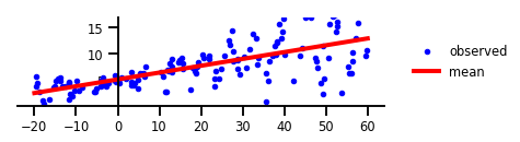
Caso 1: Sem incerteza
# Build model.
model = tf.keras.Sequential([
  tf.keras.layers.Dense(1),
  tfp.layers.DistributionLambda(lambda t: tfd.Normal(loc=t, scale=1)),
])

# Do inference.
model.compile(optimizer=tf.optimizers.Adam(learning_rate=0.01), loss=negloglik)
model.fit(x, y, epochs=1000, verbose=False);

# Profit.
[print(np.squeeze(w.numpy())) for w in model.weights];
yhat = model(x_tst)
assert isinstance(yhat, tfd.Distribution)
0.13032457
5.13029
Figura 1: Sem incertezas.
w = np.squeeze(model.layers[-2].kernel.numpy())
b = np.squeeze(model.layers[-2].bias.numpy())

plt.figure(figsize=[6, 1.5])  # inches
#plt.figure(figsize=[8, 5])  # inches
plt.plot(x, y, 'b.', label='observed');
plt.plot(x_tst, yhat.mean(),'r', label='mean', linewidth=4);
plt.ylim(-0.,17);
plt.yticks(np.linspace(0, 15, 4)[1:]);
plt.xticks(np.linspace(*x_range, num=9));

ax=plt.gca();
ax.xaxis.set_ticks_position('bottom')
ax.yaxis.set_ticks_position('left')
ax.spines['left'].set_position(('data', 0))
ax.spines['top'].set_visible(False)
ax.spines['right'].set_visible(False)
#ax.spines['left'].set_smart_bounds(True)
#ax.spines['bottom'].set_smart_bounds(True)
plt.legend(loc='center left', fancybox=True, framealpha=0., bbox_to_anchor=(1.05, 0.5))

plt.savefig('/tmp/fig1.png', bbox_inches='tight', dpi=300)
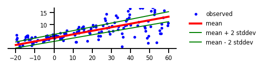
Caso 2: Incerteza Aleatórica
# Build model.
model = tf.keras.Sequential([
  tf.keras.layers.Dense(1 + 1),
  tfp.layers.DistributionLambda(
      lambda t: tfd.Normal(loc=t[..., :1],
                           scale=1e-3 + tf.math.softplus(0.05 * t[...,1:]))),
])

# Do inference.
model.compile(optimizer=tf.optimizers.Adam(learning_rate=0.01), loss=negloglik)
model.fit(x, y, epochs=1000, verbose=False);

# Profit.
[print(np.squeeze(w.numpy())) for w in model.weights];
yhat = model(x_tst)
assert isinstance(yhat, tfd.Distribution)
[0.14738432 0.1815331 ]
[4.4812164 1.2219843]
Figura 2: Incerteza Aleatórica
plt.figure(figsize=[6, 1.5])  # inches
plt.plot(x, y, 'b.', label='observed');

m = yhat.mean()
s = yhat.stddev()

plt.plot(x_tst, m, 'r', linewidth=4, label='mean');
plt.plot(x_tst, m + 2 * s, 'g', linewidth=2, label=r'mean + 2 stddev');
plt.plot(x_tst, m - 2 * s, 'g', linewidth=2, label=r'mean - 2 stddev');

plt.ylim(-0.,17);
plt.yticks(np.linspace(0, 15, 4)[1:]);
plt.xticks(np.linspace(*x_range, num=9));

ax=plt.gca();
ax.xaxis.set_ticks_position('bottom')
ax.yaxis.set_ticks_position('left')
ax.spines['left'].set_position(('data', 0))
ax.spines['top'].set_visible(False)
ax.spines['right'].set_visible(False)
#ax.spines['left'].set_smart_bounds(True)
#ax.spines['bottom'].set_smart_bounds(True)
plt.legend(loc='center left', fancybox=True, framealpha=0., bbox_to_anchor=(1.05, 0.5))

plt.savefig('/tmp/fig2.png', bbox_inches='tight', dpi=300)
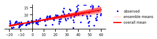
Caso 3: Incerteza Epistêmica
# Specify the surrogate posterior over `keras.layers.Dense` `kernel` and `bias`.
def posterior_mean_field(kernel_size, bias_size=0, dtype=None):
  n = kernel_size + bias_size
  c = np.log(np.expm1(1.))
  return tf.keras.Sequential([
      tfp.layers.VariableLayer(2 * n, dtype=dtype),
      tfp.layers.DistributionLambda(lambda t: tfd.Independent(
          tfd.Normal(loc=t[..., :n],
                     scale=1e-5 + tf.nn.softplus(c + t[..., n:])),
          reinterpreted_batch_ndims=1)),
  ])
# Specify the prior over `keras.layers.Dense` `kernel` and `bias`.
def prior_trainable(kernel_size, bias_size=0, dtype=None):
  n = kernel_size + bias_size
  return tf.keras.Sequential([
      tfp.layers.VariableLayer(n, dtype=dtype),
      tfp.layers.DistributionLambda(lambda t: tfd.Independent(
          tfd.Normal(loc=t, scale=1),
          reinterpreted_batch_ndims=1)),
  ])
# Build model.
model = tf.keras.Sequential([
  tfp.layers.DenseVariational(1, posterior_mean_field, prior_trainable, kl_weight=1/x.shape[0]),
  tfp.layers.DistributionLambda(lambda t: tfd.Normal(loc=t, scale=1)),
])

# Do inference.
model.compile(optimizer=tf.optimizers.Adam(learning_rate=0.01), loss=negloglik)
model.fit(x, y, epochs=1000, verbose=False);

# Profit.
[print(np.squeeze(w.numpy())) for w in model.weights];
yhat = model(x_tst)
assert isinstance(yhat, tfd.Distribution)
[ 0.1387333  5.125723  -4.112224  -2.2171402]
[0.12476114 5.147452  ]
Figura 3: Incerteza epistêmica
plt.figure(figsize=[6, 1.5])  # inches
plt.clf();
plt.plot(x, y, 'b.', label='observed');

yhats = [model(x_tst) for _ in range(100)]
avgm = np.zeros_like(x_tst[..., 0])
for i, yhat in enumerate(yhats):
  m = np.squeeze(yhat.mean())
  s = np.squeeze(yhat.stddev())
  if i < 25:
    plt.plot(x_tst, m, 'r', label='ensemble means' if i == 0 else None, linewidth=0.5)
  avgm += m
plt.plot(x_tst, avgm/len(yhats), 'r', label='overall mean', linewidth=4)

plt.ylim(-0.,17);
plt.yticks(np.linspace(0, 15, 4)[1:]);
plt.xticks(np.linspace(*x_range, num=9));

ax=plt.gca();
ax.xaxis.set_ticks_position('bottom')
ax.yaxis.set_ticks_position('left')
ax.spines['left'].set_position(('data', 0))
ax.spines['top'].set_visible(False)
ax.spines['right'].set_visible(False)
#ax.spines['left'].set_smart_bounds(True)
#ax.spines['bottom'].set_smart_bounds(True)
plt.legend(loc='center left', fancybox=True, framealpha=0., bbox_to_anchor=(1.05, 0.5))

plt.savefig('/tmp/fig3.png', bbox_inches='tight', dpi=300)
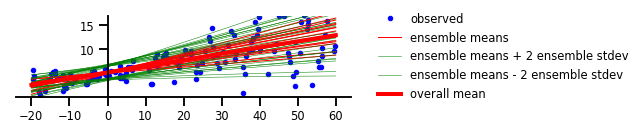
Caso 4: Incerteza Aleatórica e Epistêmica
# Build model.
model = tf.keras.Sequential([
  tfp.layers.DenseVariational(1 + 1, posterior_mean_field, prior_trainable, kl_weight=1/x.shape[0]),
  tfp.layers.DistributionLambda(
      lambda t: tfd.Normal(loc=t[..., :1],
                           scale=1e-3 + tf.math.softplus(0.01 * t[...,1:]))),
])

# Do inference.
model.compile(optimizer=tf.optimizers.Adam(learning_rate=0.01), loss=negloglik)
model.fit(x, y, epochs=1000, verbose=False);

# Profit.
[print(np.squeeze(w.numpy())) for w in model.weights];
yhat = model(x_tst)
assert isinstance(yhat, tfd.Distribution)
[ 0.12753433  2.7504077   5.160624    3.8251898  -3.4283297  -0.8961645
 -2.2378397   0.1496858 ]
[0.14511648 2.7104297  5.1248145  3.7724588 ]
Figura 4: Incerteza tanto Aleatórica quanto Epistêmica
plt.figure(figsize=[6, 1.5])  # inches
plt.plot(x, y, 'b.', label='observed');

yhats = [model(x_tst) for _ in range(100)]
avgm = np.zeros_like(x_tst[..., 0])
for i, yhat in enumerate(yhats):
  m = np.squeeze(yhat.mean())
  s = np.squeeze(yhat.stddev())
  if i < 15:
    plt.plot(x_tst, m, 'r', label='ensemble means' if i == 0 else None, linewidth=1.)
    plt.plot(x_tst, m + 2 * s, 'g', linewidth=0.5, label='ensemble means + 2 ensemble stdev' if i == 0 else None);
    plt.plot(x_tst, m - 2 * s, 'g', linewidth=0.5, label='ensemble means - 2 ensemble stdev' if i == 0 else None);
  avgm += m
plt.plot(x_tst, avgm/len(yhats), 'r', label='overall mean', linewidth=4)

plt.ylim(-0.,17);
plt.yticks(np.linspace(0, 15, 4)[1:]);
plt.xticks(np.linspace(*x_range, num=9));

ax=plt.gca();
ax.xaxis.set_ticks_position('bottom')
ax.yaxis.set_ticks_position('left')
ax.spines['left'].set_position(('data', 0))
ax.spines['top'].set_visible(False)
ax.spines['right'].set_visible(False)
#ax.spines['left'].set_smart_bounds(True)
#ax.spines['bottom'].set_smart_bounds(True)
plt.legend(loc='center left', fancybox=True, framealpha=0., bbox_to_anchor=(1.05, 0.5))

plt.savefig('/tmp/fig4.png', bbox_inches='tight', dpi=300)
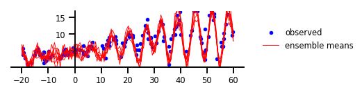
Caso 5: Incerteza funcional
Kernel PSD personalizado
class RBFKernelFn(tf.keras.layers.Layer):
  def __init__(self, **kwargs):
    super(RBFKernelFn, self).__init__(**kwargs)
    dtype = kwargs.get('dtype', None)

    self._amplitude = self.add_variable(
            initializer=tf.constant_initializer(0),
            dtype=dtype,
            name='amplitude')

    self._length_scale = self.add_variable(
            initializer=tf.constant_initializer(0),
            dtype=dtype,
            name='length_scale')

  def call(self, x):
    # Never called -- this is just a layer so it can hold variables
    # in a way Keras understands.
    return x

  @property
  def kernel(self):
    return tfp.math.psd_kernels.ExponentiatedQuadratic(
      amplitude=tf.nn.softplus(0.1 * self._amplitude),
      length_scale=tf.nn.softplus(5. * self._length_scale)
    )
# For numeric stability, set the default floating-point dtype to float64
tf.keras.backend.set_floatx('float64')

# Build model.
num_inducing_points = 40
model = tf.keras.Sequential([
    tf.keras.layers.InputLayer(input_shape=[1]),
    tf.keras.layers.Dense(1, kernel_initializer='ones', use_bias=False),
    tfp.layers.VariationalGaussianProcess(
        num_inducing_points=num_inducing_points,
        kernel_provider=RBFKernelFn(),
        event_shape=[1],
        inducing_index_points_initializer=tf.constant_initializer(
            np.linspace(*x_range, num=num_inducing_points,
                        dtype=x.dtype)[..., np.newaxis]),
        unconstrained_observation_noise_variance_initializer=(
            tf.constant_initializer(np.array(0.54).astype(x.dtype))),
    ),
])

# Do inference.
batch_size = 32
loss = lambda y, rv_y: rv_y.variational_loss(
    y, kl_weight=np.array(batch_size, x.dtype) / x.shape[0])
model.compile(optimizer=tf.optimizers.Adam(learning_rate=0.01), loss=loss)
model.fit(x, y, batch_size=batch_size, epochs=1000, verbose=False)

# Profit.
yhat = model(x_tst)
assert isinstance(yhat, tfd.Distribution)
Figura 5: Incerteza funcional
y, x, _ = load_dataset()

plt.figure(figsize=[6, 1.5])  # inches
plt.plot(x, y, 'b.', label='observed');

num_samples = 7
for i in range(num_samples):
  sample_ = yhat.sample().numpy()
  plt.plot(x_tst,
           sample_[..., 0].T,
           'r',
           linewidth=0.9,
           label='ensemble means' if i == 0 else None);

plt.ylim(-0.,17);
plt.yticks(np.linspace(0, 15, 4)[1:]);
plt.xticks(np.linspace(*x_range, num=9));

ax=plt.gca();
ax.xaxis.set_ticks_position('bottom')
ax.yaxis.set_ticks_position('left')
ax.spines['left'].set_position(('data', 0))
ax.spines['top'].set_visible(False)
ax.spines['right'].set_visible(False)
#ax.spines['left'].set_smart_bounds(True)
#ax.spines['bottom'].set_smart_bounds(True)
plt.legend(loc='center left', fancybox=True, framealpha=0., bbox_to_anchor=(1.05, 0.5))

plt.savefig('/tmp/fig5.png', bbox_inches='tight', dpi=300)