Data preprocessing for ML with Google Cloud

This tutorial shows you how to use TensorFlow Transform (the tf.Transform library) to implement data preprocessing for machine learning (ML). The tf.Transform library for TensorFlow lets you define both instance-level and full-pass data transformations through data preprocessing pipelines. These pipelines are efficiently executed with Apache Beam and they create as byproducts a TensorFlow graph to apply the same transformations during prediction as when the model is served.

This tutorial provides an end-to-end example using Dataflow as a runner for Apache Beam. It assumes that you're familiar with BigQuery, Dataflow, Vertex AI, and the TensorFlow Keras API. It also assumes that you have some experience using Jupyter Notebooks, such as with Vertex AI Workbench.

This tutorial also assumes that you're familiar with the concepts of preprocessing types, challenges, and options on Google Cloud, as described in Data preprocessing for ML: options and recommendations.

Objectives

Implement the Apache Beam pipeline using the tf.Transform library.
Run the pipeline in Dataflow.
Implement the TensorFlow model using the tf.Transform library.
Train and use the model for predictions.

Costs

This tutorial uses the following billable components of Google Cloud:

To estimate the cost to run this tutorial, assuming you use every resource for an entire day, use the preconfigured pricing calculator.

Before you begin

In the Google Cloud console, on the project selector page, select or create a Google Cloud project.

Note: If you don't plan to keep the resources that you create in this procedure, create a project instead of selecting an existing project. After you finish these steps, you can delete the project, removing all resources associated with the project.

Go to project selector
Make sure that billing is enabled for your Cloud project. Learn how to check if billing is enabled on a project.
Enable the Dataflow, Vertex AI, and Notebooks APIs. Enable the APIs

Jupyter notebooks for this solution

The following Jupyter notebooks show the implementation example:

Notebook 1 covers data preprocessing. Details are provided in the Implementing the Apache Beam pipeline section later.
Notebook 2 covers model training. Details are provided in the Implementing the TensorFlow model section later.

In the following sections, you clone these notebooks, and then you execute the notebooks to learn how the implementation example works.

Launch a user-managed notebooks instance

In the Google Cloud console, go to the Vertex AI Workbench page.

Go to Workbench
On the User-managed notebooks tab, click +New notebook.
Select TensorFlow Enterprise 2.8 (with LTS) without GPUs for the instance type.
Click Create.

After you create the notebook, wait for the proxy to JupyterLab to finish initializing. When it's ready, Open JupyterLab is displayed next to the notebook name.

Clone the notebook

On the User-managed notebooks tab, next to the notebook name, click Open JupyterLab. The JupyterLab interface opens in a new tab.

If the JupyterLab displays a Build Recommended dialog, click Cancel to reject the suggested build.
On the Launcher tab, click Terminal.

In the terminal window, clone the notebook:

git clone https://github.com/GoogleCloudPlatform/training-data-analyst

Implement the Apache Beam pipeline

This section and the next section Run the pipeline in Dataflow provide an overview and context for Notebook 1. The notebook provides a practical example to describe how to use the tf.Transform library to preprocess data. This example uses the Natality dataset, which is used to predict baby weights based on various inputs. The data is stored in the public natality table in BigQuery.

Run Notebook 1

In the JupyterLab interface, click File > Open from path, and then enter the following path:
```
training-data-analyst/blogs/babyweight_tft/babyweight_tft_keras_01.ipynb
```
Click Edit > Clear all outputs.
In the Install required packages section, execute the first cell to run the pip install apache-beam command.

The last part of the output is the following:
```
Successfully installed ...
```
You can ignore dependency errors in the output. You don't need to restart the kernel yet.
Execute the second cell to run the pip install tensorflow-transformcommand. The last part of the output is the following:
```
Successfully installed ...
Note: you may need to restart the kernel to use updated packages.
```
You can ignore dependency errors in the output.
Click Kernel > Restart Kernel.
Execute the cells in the Confirm the installed packages and Create setup.py to install packages to Dataflow containers sections.
In the Set global flags section, next to PROJECT and BUCKET, replace your-project with your Cloud project ID, and then execute the cell.
Execute all of the remaining cells through the last cell in the notebook. For information about what to do in each cell, see the instructions in the notebook.

Overview of the pipeline

In the notebook example, Dataflow runs the tf.Transform pipeline at scale to prepare the data and produce the transformation artifacts. Later sections in this document describe the functions that perform each step in the pipeline. The overall pipeline steps are as follows:

Read training data from BigQuery.
Analyze and transform training data using the tf.Transform library.
Write transformed training data to Cloud Storage in the TFRecord format.
Read evaluation data from BigQuery.
Transform evaluation data using the transform_fn graph produced by step 2.
Write transformed training data to Cloud Storage in the TFRecord format.
Write transformation artifacts to Cloud Storage that will be used later for creating and exporting the model.

The following example shows the Python code for the overall pipeline. The sections that follow provide explanations and code listings for each step.

def run_transformation_pipeline(args):

    pipeline_options = beam.pipeline.PipelineOptions(flags=[], **args)

    runner = args['runner']
    data_size = args['data_size']
    transformed_data_location = args['transformed_data_location']
    transform_artefact_location = args['transform_artefact_location']
    temporary_dir = args['temporary_dir']
    debug = args['debug']

    # Instantiate the pipeline
    with beam.Pipeline(runner, options=pipeline_options) as pipeline:
        with impl.Context(temporary_dir):

            # Preprocess train data
            step = 'train'
            # Read raw train data from BigQuery
            raw_train_dataset = read_from_bq(pipeline, step, data_size)
            # Analyze and transform raw_train_dataset
            transformed_train_dataset, transform_fn = analyze_and_transform(raw_train_dataset, step)
            # Write transformed train data to sink as tfrecords
            write_tfrecords(transformed_train_dataset, transformed_data_location, step)

            # Preprocess evaluation data
            step = 'eval'
            # Read raw eval data from BigQuery
            raw_eval_dataset = read_from_bq(pipeline, step, data_size)
            # Transform eval data based on produced transform_fn
            transformed_eval_dataset = transform(raw_eval_dataset, transform_fn, step)
            # Write transformed eval data to sink as tfrecords
            write_tfrecords(transformed_eval_dataset, transformed_data_location, step)

            # Write transformation artefacts
            write_transform_artefacts(transform_fn, transform_artefact_location)

            # (Optional) for debugging, write transformed data as text
            step = 'debug'
            # Write transformed train data as text if debug enabled
            if debug == True:
                write_text(transformed_train_dataset, transformed_data_location, step)

Read raw training data from BigQuery

The first step is to read the raw training data from BigQuery using the read_from_bq function. This function returns a raw_dataset object that is extracted from BigQuery. You pass a data_size value and pass a step value of train or eval. The BigQuery source query is constructed using the get_source_query function, as shown in the following example:

def read_from_bq(pipeline, step, data_size):

    source_query = get_source_query(step, data_size)
    raw_data = (
        pipeline
        | '{} - Read Data from BigQuery'.format(step) >> beam.io.Read(
                           beam.io.BigQuerySource(query=source_query, use_standard_sql=True))
        | '{} - Clean up Data'.format(step) >> beam.Map(prep_bq_row)
    )

    raw_metadata = create_raw_metadata()
    raw_dataset = (raw_data, raw_metadata)
    return raw_dataset

Before you perform the tf.Transform preprocessing, you might need to perform typical Apache Beam-based processing, including Map, Filter, Group, and Window processing. In the example, the code cleans the records read from BigQuery using the beam.Map(prep_bq_row) method, where prep_bq_row is a custom function. This custom function converts the numeric code for a categorical feature into human-readable labels.

In addition, to use the tf.Transform library to analyze and transform the raw_data object extracted from BigQuery, you need to create a raw_dataset object, which is a tuple of raw_data and raw_metadata objects. The raw_metadata object is created using the create_raw_metadata function, as follows:

CATEGORICAL_FEATURE_NAMES = ['is_male', 'mother_race']
NUMERIC_FEATURE_NAMES = ['mother_age', 'plurality', 'gestation_weeks']
TARGET_FEATURE_NAME = 'weight_pounds'

def create_raw_metadata():

    feature_spec = dict(
        [(name, tf.io.FixedLenFeature([], tf.string)) for name in CATEGORICAL_FEATURE_NAMES] +
        [(name, tf.io.FixedLenFeature([], tf.float32)) for name in NUMERIC_FEATURE_NAMES] +
        [(TARGET_FEATURE_NAME, tf.io.FixedLenFeature([], tf.float32))])

    raw_metadata = dataset_metadata.DatasetMetadata(
        schema_utils.schema_from_feature_spec(feature_spec))

    return raw_metadata

When you execute the cell in the notebook that immediately follows the cell that defines this method, the content of the raw_metadata.schema object is displayed. It includes the following columns:

gestation_weeks (type: FLOAT)
is_male (type: BYTES)
mother_age (type: FLOAT)
mother_race (type: BYTES)
plurality (type: FLOAT)
weight_pounds (type: FLOAT)

Transform raw training data

Imagine that you want to apply typical preprocessing transformations to the input raw features of the training data in order to prepare it for ML. These transformations include both full-pass and instance-level operations, as shown in the following table:

Input feature	Transformation	Stats needed	Type	Output feature
`weight_pound`	None	None	NA	`weight_pound`
`mother_age`	Normalize	mean, var	Full-pass	`mother_age_normalized`
`mother_age`	Equal size bucketization	quantiles	Full-pass	`mother_age_bucketized`
`mother_age`	Compute the log	None	Instance-level	`mother_age_log`
`plurality`	Indicate if it is single or multiple babies	None	Instance-level	`is_multiple`
`is_multiple`	Convert nominal values to numerical index	vocab	Full-pass	`is_multiple_index`
`gestation_weeks`	Scale between 0 and 1	min, max	Full-pass	`gestation_weeks_scaled`
`mother_race`	Convert nominal values to numerical index	vocab	Full-pass	`mother_race_index`
`is_male`	Convert nominal values to numerical index	vocab	Full-pass	`is_male_index`

These transformations are implemented in a preprocess_fn function, which expects a dictionary of tensors (input_features) and returns a dictionary of processed features (output_features).

The following code shows the implementation of the preprocess_fn function, using the tf.Transform full-pass transformation APIs (prefixed with tft.), and TensorFlow (prefixed with tf.) instance-level operations:

def preprocess_fn(input_features):

    output_features = {}

    # target feature
    output_features['weight_pounds'] = input_features['weight_pounds']

    # normalization
    output_features['mother_age_normalized'] = tft.scale_to_z_score(input_features['mother_age'])

    # scaling
    output_features['gestation_weeks_scaled'] =  tft.scale_to_0_1(input_features['gestation_weeks'])

    # bucketization based on quantiles
    output_features['mother_age_bucketized'] = tft.bucketize(input_features['mother_age'], num_buckets=5)

    # you can compute new features based on custom formulas
    output_features['mother_age_log'] = tf.math.log(input_features['mother_age'])

    # or create flags/indicators
    is_multiple = tf.as_string(input_features['plurality'] > tf.constant(1.0))

    # convert categorical features to indexed vocab
    output_features['mother_race_index'] = tft.compute_and_apply_vocabulary(input_features['mother_race'], vocab_filename='mother_race')
    output_features['is_male_index'] = tft.compute_and_apply_vocabulary(input_features['is_male'], vocab_filename='is_male')
    output_features['is_multiple_index'] = tft.compute_and_apply_vocabulary(is_multiple, vocab_filename='is_multiple')

    return output_features

The tf.Transform framework has several other transformations in addition to those in the preceding example, including those listed in the following table:

Transformation	Applies to	Description
`scale_by_min_max`	Numeric features	Scales a numerical column into the range [`output_min`, `output_max`]
`scale_to_0_1`	Numeric features	Returns a column which is the input column scaled to have range [`0`,`1`]
`scale_to_z_score`	Numeric features	Returns a standardized column with mean 0 and variance 1
`tfidf`	Text features	Maps the terms in x to their term frequency * inverse document frequency
`compute_and_apply_vocabulary`	Categorical features	Generates a vocabulary for a categorical feature and maps it to an integer with this vocab
`ngrams`	Text features	Creates a `SparseTensor` of n-grams
`hash_strings`	Categorical features	Hashes strings into buckets
`pca`	Numeric features	Computes PCA on the dataset using biased covariance
`bucketize`	Numeric features	Returns an equal-sized (quantiles-based) bucketized column, with a bucket index assigned to each input

In order to apply the transformations implemented in the preprocess_fn function to the raw_train_dataset object produced in the previous step of the pipeline, you use the AnalyzeAndTransformDataset method. This method expects the raw_dataset object as input, applies the preprocess_fn function, and it produces the transformed_dataset object and the transform_fn graph. The following code illustrates this processing:

def analyze_and_transform(raw_dataset, step):

    transformed_dataset, transform_fn = (
        raw_dataset
        | '{} - Analyze & Transform'.format(step) >> tft_beam.AnalyzeAndTransformDataset(
            preprocess_fn, output_record_batches=True)
    )

    return transformed_dataset, transform_fn

The transformations are applied on the raw data in two phases: the analyze phase and the transform phase. Figure 3 later in this document shows how the AnalyzeAndTransformDataset method is decomposed to the AnalyzeDataset method and the TransformDataset method.

The analyze phase

In the analyze phase, the raw training data is analyzed in a full-pass process to compute the statistics that are needed for the transformations. This includes computing the mean, variance, minimum, maximum, quantiles, and vocabulary. The analyze process expects a raw dataset (raw data plus raw metadata), and it produces two outputs:

transform_fn: a TensorFlow graph that contains the computed stats from the analyze phase and the transformation logic (which uses the stats) as instance-level operations. As discussed later in Save the graph, the transform_fn graph is saved to be attached to the model serving_fn function. This makes it possible to apply the same transformation to the online prediction data points.
transform_metadata: an object that describes the expected schema of the data after transformation.

The analyze phase is illustrated in the following diagram, figure 1:

The tf.Transform analyze phase. — **Figure 1.** The `tf.Transform` analyze phase.

The tf.Transform analyzers include min, max, sum, size, mean, var, covariance, quantiles, vocabulary, and pca.

The transform phase

In the transform phase, the transform_fn graph that's produced by the analyze phase is used to transform the raw training data in an instance-level process in order to produce the transformed training data. The transformed training data is paired with the transformed metadata (produced by the analyze phase) to produce the transformed_train_dataset dataset.

The transform phase is illustrated in the following diagram, figure 2:

The tf.Transform transform phase. — **Figure 2.** The `tf.Transform` transform phase.

To preprocess the features, you call the required tensorflow_transform transformations (imported as tft in the code) in your implementation of the preprocess_fn function. For example, when you call the tft.scale_to_z_score operations, the tf.Transform library translates this function call into mean and variance analyzers, computes the stats in the analyze phase, and then applies these stats to normalize the numeric feature in the transform phase. This is all done automatically by calling the AnalyzeAndTransformDataset(preprocess_fn) method.

The transformed_metadata.schema entity produced by this call includes the following columns:

gestation_weeks_scaled (type: FLOAT)
is_male_index (type: INT, is_categorical: True)
is_multiple_index (type: INT, is_categorical: True)
mother_age_bucketized (type: INT, is_categorical: True)
mother_age_log (type: FLOAT)
mother_age_normalized (type: FLOAT)
mother_race_index (type: INT, is_categorical: True)
weight_pounds (type: FLOAT)

As explained in Preprocessing operations in the first part of this series, the feature transformation converts categorical features to a numeric representation. After the transformation, the categorical features are represented by integer values. In the transformed_metadata.schema entity, the is_categorical flag for INT type columns indicates whether the column represents a categorical feature or a true numeric feature.

Write transformed training data

After the training data is preprocessed with the preprocess_fn function through the analyze and transform phases, you can write the data to a sink to be used for training the TensorFlow model. When you execute the Apache Beam pipeline using Dataflow, the sink is Cloud Storage. Otherwise, the sink is the local disk. Although you can write the data as a CSV file of fixed-width formatted files, the recommended file format for TensorFlow datasets is the TFRecord format. This is a simple record-oriented binary format that consists of tf.train.Example protocol buffer messages.

Each tf.train.Example record contains one or more features. These are converted into tensors when they are fed to the model for training. The following code writes the transformed dataset to TFRecord files in the specified location:

def write_tfrecords(transformed_dataset, location, step):
    from tfx_bsl.coders import example_coder

    transformed_data, transformed_metadata = transformed_dataset
    (
        transformed_data
        | '{} - Encode Transformed Data'.format(step) >> beam.FlatMapTuple(
                            lambda batch, _: example_coder.RecordBatchToExamples(batch))
        | '{} - Write Transformed Data'.format(step) >> beam.io.WriteToTFRecord(
                            file_path_prefix=os.path.join(location,'{}'.format(step)),
                            file_name_suffix='.tfrecords')
    )

Read, transform, and write evaluation data

After you transform the training data and produce the transform_fn graph, you can use it to transform the evaluation data. First, you read and clean the evaluation data from BigQuery using the read_from_bq function described earlier in Read raw training data from BigQuery, and passing a value of eval for the step parameter. Then, you use the following code to transform the raw evaluation dataset (raw_dataset) to the expected transformed format (transformed_dataset):

def transform(raw_dataset, transform_fn, step):

    transformed_dataset = (
        (raw_dataset, transform_fn)
        | '{} - Transform'.format(step) >> tft_beam.TransformDataset(output_record_batches=True)
    )

    return transformed_dataset

When you transform the evaluation data, only instance-level operations apply, using both the logic in the transform_fn graph and the statistics computed from the analyze phase in the training data. In other words, you don't analyze the evaluation data in a full-pass fashion to compute new statistics, like the mean and the variance for z-score normalization of numeric features in evaluation data. Instead, you use the computed statistics from the training data to transform the evaluation data in an instance-level fashion.

Therefore, you use the AnalyzeAndTransform method in the context of training data to compute the statistics and transform the data. At the same time, you use the TransformDataset method in the context of transforming evaluation data to only transform the data using the statistics computed on the training data.

You then write the data to a sink (Cloud Storage or local disk, depending on the runner) in the TFRecord format for evaluating the TensorFlow model during the training process. To do this, you use the write_tfrecords function that's discussed in Write transformed training data. The following diagram, figure 3, shows how the transform_fn graph that's produced in the analyze phase of the training data is used to transform the evaluation data.

Transforming evaluation data using the transform_fn graph. — **Figure 3.** Transforming evaluation data using the `transform_fn` graph.

Save the graph

A final step in the tf.Transform preprocessing pipeline is to store the artifacts, which includes the transform_fn graph that's produced by the analyze phase on the training data. The code for storing the artifacts is shown in the following write_transform_artefacts function:

def write_transform_artefacts(transform_fn, location):

    (
        transform_fn
        | 'Write Transform Artifacts' >> transform_fn_io.WriteTransformFn(location)
    )

These artifacts will be used later for model training and exporting for serving. The following artifacts are also produced, as shown in the next section:

saved_model.pb: represents the TensorFlow graph that includes the transformation logic (the transform_fn graph), which is to be attached to the model serving interface to transform the raw data points to the transformed format.
variables: includes the statistics computed during the analyze phase of the training data, and is used in the transformation logic in the saved_model.pb artifact.
assets: includes vocabulary files, one for each categorical feature processed with the compute_and_apply_vocabulary method, to be used during serving to convert an input raw nominal value to a numerical index.
transformed_metadata: a directory that contains the schema.json file that describes the schema of the transformed data.

Run the pipeline in Dataflow

After you define the tf.Transform pipeline, you run the pipeline using Dataflow. The following diagram, figure 4, shows the Dataflow execution graph of the tf.Transform pipeline described in the example.

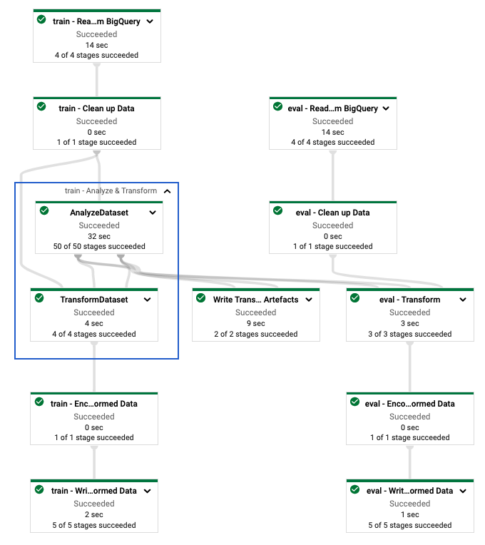
Dataflow execution graph of the tf.Transform pipeline. — **Figure 4.** Dataflow execution graph of the `tf.Transform` pipeline.

After you execute the Dataflow pipeline to preprocess the training and evaluation data, you can explore the produced objects in Cloud Storage by executing the last cell in the notebook. The code snippets in this section show the results, where YOUR_BUCKET_NAME is the name of your Cloud Storage bucket.

The transformed training and evaluation data in TFRecord format are stored at the following location:

gs://YOUR_BUCKET_NAME/babyweight_tft/transformed

The transform artifacts are produced at the following location:

gs://YOUR_BUCKET_NAME/babyweight_tft/transform

The following list is the output of the pipeline, showing the produced data objects and artifacts:

transformed data:
gs://YOUR_BUCKET_NAME/babyweight_tft/transformed/eval-00000-of-00001.tfrecords
gs://YOUR_BUCKET_NAME/babyweight_tft/transformed/train-00000-of-00002.tfrecords
gs://YOUR_BUCKET_NAME/babyweight_tft/transformed/train-00001-of-00002.tfrecords

transformed metadata:
gs://YOUR_BUCKET_NAME/babyweight_tft/transform/transformed_metadata/
gs://YOUR_BUCKET_NAME/babyweight_tft/transform/transformed_metadata/asset_map
gs://YOUR_BUCKET_NAME/babyweight_tft/transform/transformed_metadata/schema.pbtxt

transform artefact:
gs://YOUR_BUCKET_NAME/babyweight_tft/transform/transform_fn/
gs://YOUR_BUCKET_NAME/babyweight_tft/transform/transform_fn/saved_model.pb
gs://YOUR_BUCKET_NAME/babyweight_tft/transform/transform_fn/assets/
gs://YOUR_BUCKET_NAME/babyweight_tft/transform/transform_fn/variables/

transform assets:
gs://YOUR_BUCKET_NAME/babyweight_tft/transform/transform_fn/assets/
gs://YOUR_BUCKET_NAME/babyweight_tft/transform/transform_fn/assets/is_male
gs://YOUR_BUCKET_NAME/babyweight_tft/transform/transform_fn/assets/is_multiple
gs://YOUR_BUCKET_NAME/babyweight_tft/transform/transform_fn/assets/mother_race

Implement the TensorFlow model

This section and the next section, Train and use the model for predictions, provide an overview and context for Notebook 2. The notebook provides an example ML model to predict baby weights. In this example, a TensorFlow model is implemented using the Keras API. The model uses the data and artifacts that are produced by the tf.Transform preprocessing pipeline explained earlier.

Run Notebook 2

In the JupyterLab interface, click File > Open from path, and then enter the following path:
```
training-data-analyst/blogs/babyweight_tft/babyweight_tft_keras_02.ipynb
```
Click Edit > Clear all outputs.
In the Install required packages section, execute the first cell to run the pip install tensorflow-transform command.

The last part of the output is the following:
```
Successfully installed ...
Note: you may need to restart the kernel to use updated packages.
```
You can ignore dependency errors in the output.
In the Kernel menu, select Restart Kernel.
Execute the cells in the Confirm the installed packages and Create setup.py to install packages to Dataflow containers sections.
In the Set global flags section, next to PROJECT and BUCKET, replace your-project with your Cloud project ID, and then execute the cell.
Execute all of the remaining cells through the last cell in the notebook. For information about what to do in each cell, see the instructions in the notebook.

Overview of the model creation

The steps for creating the model are as follows:

Create feature columns using the schema information that is stored in the transformed_metadata directory.
Create the wide and deep model with the Keras API using the feature columns as input to the model.
Create the tfrecords_input_fn function to read and parse the training and evaluation data using the transform artifacts.
Train and evaluate the model.
Export the trained model by defining a serving_fn function that has the transform_fn graph attached to it.
Inspect the exported model using the saved_model_cli tool.
Use the exported model for prediction.

This document doesn't explain how to build the model, so it doesn't discuss in detail how the model was built or trained. However, the following sections show how the information stored in the transform_metadata directory—which is produced by the tf.Transform process—is used to create the feature columns of the model. The document also shows how the transform_fn graph—which is also produced by tf.Transform process—is used in the serving_fn function when the model is exported for serving.

Use the generated transform artifacts in model training

When you train the TensorFlow model, you use the transformed train and eval objects produced in the previous data processing step. These objects are stored as sharded files in the TFRecord format. The schema information in the transformed_metadata directory generated in the previous step can be useful in parsing the data (tf.train.Example objects) to feed into the model for training and evaluation.

Parse the data

Because you read files in the TFRecord format to feed the model with training and evaluation data, you need to parse each tf.train.Example object in the files to create a dictionary of features (tensors). This ensures that the features are mapped to the model input layer using the feature columns, which act as the model training and evaluation interface. To parse the data, you use the TFTransformOutput object that is created from the artifacts generated in the previous step:

Create a TFTransformOutput object from the artifacts that are generated and saved in the previous preprocessing step, as described in the Save the graph section:
```
tf_transform_output = tft.TFTransformOutput(TRANSFORM_ARTEFACTS_DIR)
```
Extract a feature_spec object from the TFTransformOutput object:
```
tf_transform_output.transformed_feature_spec()
```

Use the feature_spec object to specify the features contained in the tf.train.Example object as in the tfrecords_input_fn function:

def tfrecords_input_fn(files_name_pattern, batch_size=512):

    tf_transform_output = tft.TFTransformOutput(TRANSFORM_ARTEFACTS_DIR)
    TARGET_FEATURE_NAME = 'weight_pounds'

    batched_dataset = tf.data.experimental.make_batched_features_dataset(
        file_pattern=files_name_pattern,
        batch_size=batch_size,
        features=tf_transform_output.transformed_feature_spec(),
        reader=tf.data.TFRecordDataset,
        label_key=TARGET_FEATURE_NAME,
        shuffle=True).prefetch(tf.data.experimental.AUTOTUNE)

    return batched_dataset

Create the feature columns

The pipeline produces the schema information in the transformed_metadata directory that describes the schema of the transformed data that is expected by the model for training and evaluation. The schema contains the feature name and data type, such as the following:

gestation_weeks_scaled (type: FLOAT)
is_male_index (type: INT, is_categorical: True)
is_multiple_index (type: INT, is_categorical: True)
mother_age_bucketized (type: INT, is_categorical: True)
mother_age_log (type: FLOAT)
mother_age_normalized (type: FLOAT)
mother_race_index (type: INT, is_categorical: True)
weight_pounds (type: FLOAT)

To see this information, use the following commands:

transformed_metadata = tft.TFTransformOutput(TRANSFORM_ARTEFACTS_DIR).transformed_metadata
transformed_metadata.schema

The following code shows how you use the feature name to create feature columns:

def create_wide_and_deep_feature_columns():

    deep_feature_columns = []
    wide_feature_columns = []
    inputs = {}
    categorical_columns = {}

    # Select features you've checked from the metadata
    # Categorical features are associated with the vocabulary size (starting from 0)
    numeric_features = ['mother_age_log', 'mother_age_normalized', 'gestation_weeks_scaled']
    categorical_features = [('is_male_index', 1), ('is_multiple_index', 1),
                            ('mother_age_bucketized', 4), ('mother_race_index', 10)]

    for feature in numeric_features:
        deep_feature_columns.append(tf.feature_column.numeric_column(feature))
        inputs[feature] = layers.Input(shape=(), name=feature, dtype='float32')

    for feature, vocab_size in categorical_features:
        categorical_columns[feature] = (
            tf.feature_column.categorical_column_with_identity(feature, num_buckets=vocab_size+1))
        wide_feature_columns.append(tf.feature_column.indicator_column(categorical_columns[feature]))
        inputs[feature] = layers.Input(shape=(), name=feature, dtype='int64')

    mother_race_X_mother_age_bucketized = tf.feature_column.crossed_column(
        [categorical_columns['mother_age_bucketized'],
         categorical_columns['mother_race_index']],  55)
    wide_feature_columns.append(tf.feature_column.indicator_column(mother_race_X_mother_age_bucketized))

    mother_race_X_mother_age_bucketized_embedded = tf.feature_column.embedding_column(
        mother_race_X_mother_age_bucketized, 5)
    deep_feature_columns.append(mother_race_X_mother_age_bucketized_embedded)

    return wide_feature_columns, deep_feature_columns, inputs

The code creates a tf.feature_column.numeric_column column for numeric features, and a tf.feature_column.categorical_column_with_identity column for categorical features.

You can also create extended feature columns, as described in Option C: TensorFlow in the first part of this series. In the example used for this series, a new feature is created, mother_race_X_mother_age_bucketized, by crossing the mother_race and mother_age_bucketized features using the tf.feature_column.crossed_column feature column. Low-dimensional, dense representation of this crossed feature is created using the tf.feature_column.embedding_column feature column.

The following diagram, figure 5, shows the transformed data and how the transformed metadata is used to define and train the TensorFlow model:

Training the TensorFlow model with transformed data. — **Figure 5.** Training the TensorFlow model with the transformed data.

Export the model for serving prediction

After you train the TensorFlow model with the Keras API, you export the trained model as a SavedModel object, so that it can serve new data points for prediction. When you export the model, you have to define its interface—that is, the input features schema that is expected during serving. This input features schema is defined in the serving_fn function, as shown in the following code:

def export_serving_model(model, output_dir):

    tf_transform_output = tft.TFTransformOutput(TRANSFORM_ARTEFACTS_DIR)
    # The layer has to be saved to the model for Keras tracking purposes.
    model.tft_layer = tf_transform_output.transform_features_layer()

    @tf.function
    def serveing_fn(uid, is_male, mother_race, mother_age, plurality, gestation_weeks):
        features = {
            'is_male': is_male,
            'mother_race': mother_race,
            'mother_age': mother_age,
            'plurality': plurality,
            'gestation_weeks': gestation_weeks
        }
        transformed_features = model.tft_layer(features)
        outputs = model(transformed_features)
        # The prediction results have multiple elements in general.
        # But we need only the first element in our case.
        outputs = tf.map_fn(lambda item: item[0], outputs)

        return {'uid': uid, 'weight': outputs}

    concrete_serving_fn = serveing_fn.get_concrete_function(
        tf.TensorSpec(shape=[None], dtype=tf.string, name='uid'),
        tf.TensorSpec(shape=[None], dtype=tf.string, name='is_male'),
        tf.TensorSpec(shape=[None], dtype=tf.string, name='mother_race'),
        tf.TensorSpec(shape=[None], dtype=tf.float32, name='mother_age'),
        tf.TensorSpec(shape=[None], dtype=tf.float32, name='plurality'),
        tf.TensorSpec(shape=[None], dtype=tf.float32, name='gestation_weeks')
    )
    signatures = {'serving_default': concrete_serving_fn}

    model.save(output_dir, save_format='tf', signatures=signatures)

During serving, the model expects the data points in their raw form (that is, raw features before transformations). Therefore, the serving_fn function receives the raw features and stores them in a features object as a Python dictionary. However, as discussed earlier, the trained model expects the data points in the transformed schema. To convert the raw features into the transformed_features objects that are expected by the model interface, you apply the saved transform_fn graph to the features object with the following steps:

Create the TFTransformOutput object from the artifacts generated and saved in the previous preprocessing step:
```
tf_transform_output = tft.TFTransformOutput(TRANSFORM_ARTEFACTS_DIR)
```
Create a TransformFeaturesLayer object from the TFTransformOutput object:
```
model.tft_layer = tf_transform_output.transform_features_layer()
```
Apply the transform_fn graph using the TransformFeaturesLayer object:
```
transformed_features = model.tft_layer(features)
```

The following diagram, figure 6, illustrates the final step of exporting a model for serving:

Exporting the model for serving with the transform_fn graph attached. — **Figure 6.** Exporting the model for serving with the `transform_fn` graph attached.

Train and use the model for predictions

You can train the model locally by executing the cells of the notebook. For examples of how to package the code and train your model at scale using Vertex AI Training, see the samples and guides in the Google Cloud cloudml-samples GitHub repository.

When you inspect the exported SavedModel object using the saved_model_cli tool, you see that the inputs elements of the signature definition signature_def include the raw features, as shown in the following example:

signature_def['serving_default']:
  The given SavedModel SignatureDef contains the following input(s):
    inputs['gestation_weeks'] tensor_info:
        dtype: DT_FLOAT
        shape: (-1)
        name: serving_default_gestation_weeks:0
    inputs['is_male'] tensor_info:
        dtype: DT_STRING
        shape: (-1)
        name: serving_default_is_male:0
    inputs['mother_age'] tensor_info:
        dtype: DT_FLOAT
        shape: (-1)
        name: serving_default_mother_age:0
    inputs['mother_race'] tensor_info:
        dtype: DT_STRING
        shape: (-1)
        name: serving_default_mother_race:0
    inputs['plurality'] tensor_info:
        dtype: DT_FLOAT
        shape: (-1)
        name: serving_default_plurality:0
    inputs['uid'] tensor_info:
        dtype: DT_STRING
        shape: (-1)
        name: serving_default_uid:0
  The given SavedModel SignatureDef contains the following output(s):
    outputs['uid'] tensor_info:
        dtype: DT_STRING
        shape: (-1)
        name: StatefulPartitionedCall_6:0
    outputs['weight'] tensor_info:
        dtype: DT_FLOAT
        shape: (-1)
        name: StatefulPartitionedCall_6:1
  Method name is: tensorflow/serving/predict

The remaining cells of the notebook show you how to use the exported model for a local prediction, and how to deploy the model as a microservice using Vertex AI Prediction. It is important to highlight that the input (sample) data point is in the raw schema in both cases.

Clean up

To avoid incurring additional charges to your Google Cloud account for the resources used in this tutorial, delete the project that contains the resources.

Delete the project

In the Google Cloud console, go to the Manage resources page.

Go to Manage resources
In the project list, select the project that you want to delete, and then click Delete.
In the dialog, type the project ID, and then click Shut down to delete the project.

What's next

To learn about the concepts, challenges, and options of data preprocessing for machine learning on Google Cloud, see the first article in this series, Data preprocessing for ML: options and recommendations.
For more information about how to implement, package, and run a tf.Transform pipeline on Dataflow, see the Predicting income with Census Dataset sample.
Take the Coursera specialization on ML with TensorFlow on Google Cloud.
Learn about best practices for ML engineering in Rules of ML.
For more reference architectures, diagrams, and best practices, explore the Cloud Architecture Center.