
| | |  GitHub에서 소스 보기 GitHub에서 소스 보기 | |
이 자습서에는 단어 임베딩에 대한 소개가 포함되어 있습니다. 감정 분류 작업을 위해 간단한 Keras 모델을 사용하여 자신만의 단어 임베딩을 훈련한 다음 임베딩 프로젝터 에서 시각화합니다(아래 이미지 참조).

텍스트를 숫자로 표현하기
기계 학습 모델은 벡터(숫자 배열)를 입력으로 사용합니다. 텍스트로 작업할 때 가장 먼저 해야 할 일은 문자열을 모델에 제공하기 전에 문자열을 숫자로 변환(또는 텍스트를 "벡터화")하는 전략을 마련하는 것입니다. 이 섹션에서는 그렇게 하기 위한 세 가지 전략을 살펴볼 것입니다.
원-핫 인코딩
첫 번째 아이디어로 어휘의 각 단어를 "원 핫"으로 인코딩할 수 있습니다. "고양이가 매트 위에 앉았다"라는 문장을 생각해 보십시오. 이 문장의 어휘(또는 고유한 단어)는 (cat, mat, on, sat,)입니다. 각 단어를 나타내기 위해 길이가 어휘와 동일한 0 벡터를 만든 다음 단어에 해당하는 인덱스에 1을 배치합니다. 이 접근 방식은 다음 다이어그램에 나와 있습니다.
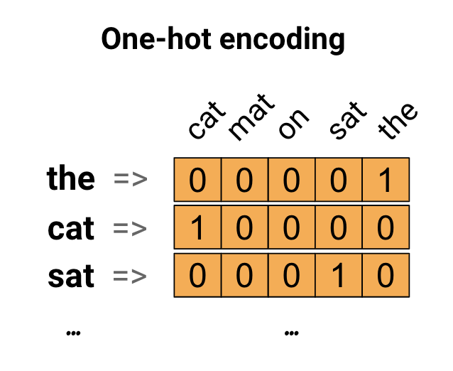
문장의 인코딩을 포함하는 벡터를 생성하기 위해 각 단어에 대한 원-핫 벡터를 연결할 수 있습니다.
고유 번호로 각 단어 인코딩
시도할 수 있는 두 번째 접근 방식은 고유 번호를 사용하여 각 단어를 인코딩하는 것입니다. 위의 예를 계속하면 "cat"에 1을 할당하고 "mat"에 2를 할당하는 식으로 계속할 수 있습니다. 그런 다음 "cat sit on the mat" 문장을 [5, 1, 4, 3, 5, 2]와 같은 밀집 벡터로 인코딩할 수 있습니다. 이 접근 방식은 효율적입니다. 희소 벡터 대신 이제 조밀한 벡터(모든 요소가 가득 찬)가 있습니다.
그러나 이 접근 방식에는 두 가지 단점이 있습니다.
정수 인코딩은 임의적입니다(단어 간의 관계를 캡처하지 않음).
정수 인코딩은 모델이 해석하기 어려울 수 있습니다. 예를 들어 선형 분류기는 각 기능에 대해 단일 가중치를 학습합니다. 두 단어의 유사성과 인코딩의 유사성 사이에는 관계가 없기 때문에 이 기능 가중치 조합은 의미가 없습니다.
단어 임베딩
단어 임베딩은 유사한 단어가 유사한 인코딩을 갖는 효율적이고 조밀한 표현을 사용하는 방법을 제공합니다. 중요한 것은 이 인코딩을 직접 지정할 필요가 없다는 것입니다. 임베딩은 부동 소수점 값의 조밀한 벡터입니다(벡터의 길이는 사용자가 지정하는 매개변수임). 임베딩에 대한 값을 수동으로 지정하는 대신 학습 가능한 매개변수입니다(모델이 조밀한 계층에 대한 가중치를 학습하는 것과 같은 방식으로 학습 중 모델에 의해 학습된 가중치). 큰 데이터 세트로 작업할 때 8차원(작은 데이터 세트의 경우), 최대 1024차원의 단어 임베딩을 보는 것이 일반적입니다. 더 높은 차원의 임베딩은 단어 간의 세분화된 관계를 캡처할 수 있지만 학습하는 데 더 많은 데이터가 필요합니다.
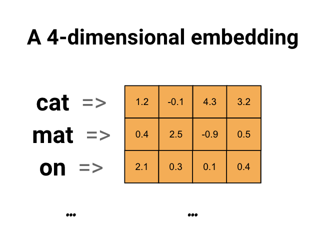
위는 단어 임베딩에 대한 다이어그램입니다. 각 단어는 부동 소수점 값의 4차원 벡터로 표시됩니다. 임베딩을 생각하는 또 다른 방법은 "룩업 테이블"입니다. 이러한 가중치를 학습한 후 테이블에서 해당하는 조밀한 벡터를 조회하여 각 단어를 인코딩할 수 있습니다.
설정
import io
import os
import re
import shutil
import string
import tensorflow as tf

from tensorflow.keras import Sequential
from tensorflow.keras.layers import Dense, Embedding, GlobalAveragePooling1D
from tensorflow.keras.layers import TextVectorization
IMDb 데이터세트 다운로드
튜토리얼을 통해 Large Movie Review Dataset 을 사용할 것입니다. 이 데이터 세트에서 감정 분류기 모델을 훈련하고 그 과정에서 처음부터 임베딩을 배웁니다. 데이터세트를 처음부터 로드하는 방법에 대해 자세히 알아보려면 텍스트 로드 튜토리얼 을 참조하세요.
Keras 파일 유틸리티를 사용하여 데이터 세트를 다운로드하고 디렉토리를 살펴보십시오.
url = "https://ai.stanford.edu/~amaas/data/sentiment/aclImdb_v1.tar.gz"

dataset = tf.keras.utils.get_file("aclImdb_v1.tar.gz", url,
                                  untar=True, cache_dir='.',
                                  cache_subdir='')

dataset_dir = os.path.join(os.path.dirname(dataset), 'aclImdb')
os.listdir(dataset_dir)
Downloading data from https://ai.stanford.edu/~amaas/data/sentiment/aclImdb_v1.tar.gz
84131840/84125825 [==============================] - 7s 0us/step
84140032/84125825 [==============================] - 7s 0us/step
['test', 'imdb.vocab', 'imdbEr.txt', 'train', 'README']
train/ 디렉토리를 살펴보십시오. 영화 리뷰가 각각 긍정 및 부정으로 표시된 pos 및 neg 폴더가 있습니다. pos 및 neg 폴더의 리뷰를 사용하여 이진 분류 모델을 훈련합니다.
train_dir = os.path.join(dataset_dir, 'train')
os.listdir(train_dir)
['urls_pos.txt',
 'urls_unsup.txt',
 'urls_neg.txt',
 'pos',
 'unsup',
 'unsupBow.feat',
 'neg',
 'labeledBow.feat']
train 디렉토리에는 훈련 데이터 세트를 생성하기 전에 제거해야 하는 추가 폴더도 있습니다.
remove_dir = os.path.join(train_dir, 'unsup')
shutil.rmtree(remove_dir)
다음으로 tf.data.Dataset 를 사용하여 tf.keras.utils.text_dataset_from_directory 을 생성합니다. 이 텍스트 분류 튜토리얼 에서 이 유틸리티 사용에 대해 자세히 알아볼 수 있습니다.
train 디렉토리를 사용하여 검증을 위해 20% 분할로 훈련 데이터 세트와 검증 데이터 세트를 모두 생성합니다.
batch_size = 1024
seed = 123
train_ds = tf.keras.utils.text_dataset_from_directory(
    'aclImdb/train', batch_size=batch_size, validation_split=0.2,
    subset='training', seed=seed)
val_ds = tf.keras.utils.text_dataset_from_directory(
    'aclImdb/train', batch_size=batch_size, validation_split=0.2,
    subset='validation', seed=seed)
Found 25000 files belonging to 2 classes.
Using 20000 files for training.
Found 25000 files belonging to 2 classes.
Using 5000 files for validation.
기차 데이터 세트에서 몇 가지 영화 리뷰와 레이블 (1: positive, 0: negative) 을 살펴보세요.
for text_batch, label_batch in train_ds.take(1):
  for i in range(5):
    print(label_batch[i].numpy(), text_batch.numpy()[i])
0 b"Oh My God! Please, for the love of all that is holy, Do Not Watch This Movie! It it 82 minutes of my life I will never get back. Sure, I could have stopped watching half way through. But I thought it might get better. It Didn't. Anyone who actually enjoyed this movie is one seriously sick and twisted individual. No wonder us Australians/New Zealanders have a terrible reputation when it comes to making movies. Everything about this movie is horrible, from the acting to the editing. I don't even normally write reviews on here, but in this case I'll make an exception. I only wish someone had of warned me before I hired this catastrophe"
1 b'This movie is SOOOO funny!!! The acting is WONDERFUL, the Ramones are sexy, the jokes are subtle, and the plot is just what every high schooler dreams of doing to his/her school. I absolutely loved the soundtrack as well as the carefully placed cynicism. If you like monty python, You will love this film. This movie is a tad bit "grease"esk (without all the annoying songs). The songs that are sung are likable; you might even find yourself singing these songs once the movie is through. This musical ranks number two in musicals to me (second next to the blues brothers). But please, do not think of it as a musical per say; seeing as how the songs are so likable, it is hard to tell a carefully choreographed scene is taking place. I think of this movie as more of a comedy with undertones of romance. You will be reminded of what it was like to be a rebellious teenager; needless to say, you will be reminiscing of your old high school days after seeing this film. Highly recommended for both the family (since it is a very youthful but also for adults since there are many jokes that are funnier with age and experience.'
0 b"Alex D. Linz replaces Macaulay Culkin as the central figure in the third movie in the Home Alone empire. Four industrial spies acquire a missile guidance system computer chip and smuggle it through an airport inside a remote controlled toy car. Because of baggage confusion, grouchy Mrs. Hess (Marian Seldes) gets the car. She gives it to her neighbor, Alex (Linz), just before the spies turn up. The spies rent a house in order to burglarize each house in the neighborhood until they locate the car. Home alone with the chicken pox, Alex calls 911 each time he spots a theft in progress, but the spies always manage to elude the police while Alex is accused of making prank calls. The spies finally turn their attentions toward Alex, unaware that he has rigged devices to cleverly booby-trap his entire house. Home Alone 3 wasn't horrible, but probably shouldn't have been made, you can't just replace Macauley Culkin, Joe Pesci, or Daniel Stern. Home Alone 3 had some funny parts, but I don't like when characters are changed in a movie series, view at own risk."
0 b"There's a good movie lurking here, but this isn't it. The basic idea is good: to explore the moral issues that would face a group of young survivors of the apocalypse. But the logic is so muddled that it's impossible to get involved.<br /><br />For example, our four heroes are (understandably) paranoid about catching the mysterious airborne contagion that's wiped out virtually all of mankind. Yet they wear surgical masks some times, not others. Some times they're fanatical about wiping down with bleach any area touched by an infected person. Other times, they seem completely unconcerned.<br /><br />Worse, after apparently surviving some weeks or months in this new kill-or-be-killed world, these people constantly behave like total newbs. They don't bother accumulating proper equipment, or food. They're forever running out of fuel in the middle of nowhere. They don't take elementary precautions when meeting strangers. And after wading through the rotting corpses of the entire human race, they're as squeamish as sheltered debutantes. You have to constantly wonder how they could have survived this long... and even if they did, why anyone would want to make a movie about them.<br /><br />So when these dweebs stop to agonize over the moral dimensions of their actions, it's impossible to take their soul-searching seriously. Their actions would first have to make some kind of minimal sense.<br /><br />On top of all this, we must contend with the dubious acting abilities of Chris Pine. His portrayal of an arrogant young James T Kirk might have seemed shrewd, when viewed in isolation. But in Carriers he plays on exactly that same note: arrogant and boneheaded. It's impossible not to suspect that this constitutes his entire dramatic range.<br /><br />On the positive side, the film *looks* excellent. It's got an over-sharp, saturated look that really suits the southwestern US locale. But that can't save the truly feeble writing nor the paper-thin (and annoying) characters. Even if you're a fan of the end-of-the-world genre, you should save yourself the agony of watching Carriers."
0 b'I saw this movie at an actual movie theater (probably the \\(2.00 one) with my cousin and uncle. We were around 11 and 12, I guess, and really into scary movies. I remember being so excited to see it because my cool uncle let us pick the movie (and we probably never got to do that again!) and sooo disappointed afterwards!! Just boring and not scary. The only redeeming thing I can remember was Corky Pigeon from Silver Spoons, and that wasn\'t all that great, just someone I recognized. I\'ve seen bad movies before and this one has always stuck out in my mind as the worst. This was from what I can recall, one of the most boring, non-scary, waste of our collective \\)6, and a waste of film. I have read some of the reviews that say it is worth a watch and I say, "Too each his own", but I wouldn\'t even bother. Not even so bad it\'s good.'
성능을 위한 데이터세트 구성
I/O가 차단되지 않도록 데이터를 로드할 때 사용해야 하는 두 가지 중요한 방법입니다.
.cache() 는 디스크에서 로드된 후 데이터를 메모리에 유지합니다. 이렇게 하면 모델을 훈련하는 동안 데이터 세트가 병목 현상이 되지 않습니다. 데이터 세트가 너무 커서 메모리에 맞지 않는 경우 이 방법을 사용하여 많은 작은 파일보다 읽기에 더 효율적인 고성능 온디스크 캐시를 생성할 수도 있습니다.
.prefetch() 는 훈련하는 동안 데이터 전처리와 모델 실행을 겹칩니다.
데이터 성능 가이드 에서 두 가지 방법과 데이터를 디스크에 캐시하는 방법에 대해 자세히 알아볼 수 있습니다.
AUTOTUNE = tf.data.AUTOTUNE

train_ds = train_ds.cache().prefetch(buffer_size=AUTOTUNE)
val_ds = val_ds.cache().prefetch(buffer_size=AUTOTUNE)
포함 레이어 사용
Keras를 사용하면 단어 임베딩을 쉽게 사용할 수 있습니다. Embedding 레이어를 살펴보십시오.
임베딩 레이어는 정수 인덱스(특정 단어를 나타냄)에서 밀집 벡터(임베딩)로 매핑하는 조회 테이블로 이해할 수 있습니다. 임베딩의 차원(또는 너비)은 Dense 레이어의 뉴런 수를 실험하는 것과 같은 방식으로 문제에 잘 맞는 것을 확인하기 위해 실험할 수 있는 매개변수입니다.
# Embed a 1,000 word vocabulary into 5 dimensions.
embedding_layer = tf.keras.layers.Embedding(1000, 5)
임베딩 레이어를 생성할 때 임베딩의 가중치는 다른 레이어와 마찬가지로 무작위로 초기화됩니다. 훈련하는 동안 역전파를 통해 점진적으로 조정됩니다. 일단 훈련되면 학습된 단어 임베딩은 단어 간의 유사성을 대략적으로 인코딩합니다(모델이 훈련된 특정 문제에 대해 학습된 대로).
임베딩 레이어에 정수를 전달하면 결과는 각 정수를 임베딩 테이블의 벡터로 대체합니다.
result = embedding_layer(tf.constant([1, 2, 3]))
result.numpy()
array([[ 0.01318491, -0.02219239,  0.024673  , -0.03208025,  0.02297195],
       [-0.00726584,  0.03731754, -0.01209557, -0.03887399, -0.02407478],
       [ 0.04477594,  0.04504738, -0.02220147, -0.03642888, -0.04688282]],
      dtype=float32)
텍스트 또는 시퀀스 문제의 경우 Embedding 레이어는 모양 (samples, sequence_length) 의 정수 2D 텐서를 사용합니다. 여기서 각 항목은 정수 시퀀스입니다. 가변 길이의 시퀀스를 포함할 수 있습니다. 모양이 (32, 10) (길이가 10인 32개 시퀀스의 배치) 또는 (64, 15) (길이가 15인 64개 시퀀스의 배치)가 있는 배치 위의 임베딩 레이어에 공급할 수 있습니다.
반환된 텐서는 입력보다 축이 하나 더 있고 임베딩 벡터는 새로운 마지막 축을 따라 정렬됩니다. (2, 3) 입력 배치에 전달하면 출력은 (2, 3, N)
result = embedding_layer(tf.constant([[0, 1, 2], [3, 4, 5]]))
result.shape
TensorShape([2, 3, 5])
시퀀스 배치가 입력으로 주어지면 임베딩 레이어는 (samples, sequence_length, embedding_dimensionality) 모양의 3D 부동 소수점 텐서를 반환합니다. 이 가변 길이 시퀀스에서 고정 표현으로 변환하기 위해 다양한 표준 접근 방식이 있습니다. Dense 계층으로 전달하기 전에 RNN, Attention 또는 pooling 계층을 사용할 수 있습니다. 이 자습서에서는 풀링이 가장 간단하기 때문에 풀링을 사용합니다. RNN 튜토리얼을 사용한 텍스트 분류 는 좋은 다음 단계입니다.
텍스트 전처리
다음으로 감정 분류 모델에 필요한 데이터 세트 사전 처리 단계를 정의합니다. 영화 리뷰를 벡터화하기 위해 원하는 매개변수로 TextVectorization 레이어를 초기화합니다. 텍스트 분류 자습서에서 이 레이어를 사용하는 방법에 대해 자세히 알아볼 수 있습니다.
# Create a custom standardization function to strip HTML break tags '<br />'.
def custom_standardization(input_data):
  lowercase = tf.strings.lower(input_data)
  stripped_html = tf.strings.regex_replace(lowercase, '<br />', ' ')
  return tf.strings.regex_replace(stripped_html,
                                  '[%s]' % re.escape(string.punctuation), '')


# Vocabulary size and number of words in a sequence.
vocab_size = 10000
sequence_length = 100

# Use the text vectorization layer to normalize, split, and map strings to
# integers. Note that the layer uses the custom standardization defined above.
# Set maximum_sequence length as all samples are not of the same length.
vectorize_layer = TextVectorization(
    standardize=custom_standardization,
    max_tokens=vocab_size,
    output_mode='int',
    output_sequence_length=sequence_length)

# Make a text-only dataset (no labels) and call adapt to build the vocabulary.
text_ds = train_ds.map(lambda x, y: x)
vectorize_layer.adapt(text_ds)
분류 모델 만들기
Keras Sequential API 를 사용하여 감정 분류 모델을 정의합니다. 이 경우 "Continuous Bag of Words" 스타일 모델입니다.
-
TextVectorization레이어는 문자열을 어휘 인덱스로 변환합니다. 이미vectorize_layer를 TextVectorization 레이어로 초기화하고text_ds에서adapt을 호출하여 해당 어휘를 구축했습니다. 이제 vectorize_layer를 종단 간 분류 모델의 첫 번째 계층으로 사용하여 변환된 문자열을 Embedding 계층에 공급할 수 있습니다. Embedding레이어는 정수로 인코딩된 어휘를 취하고 각 단어 인덱스에 대한 임베딩 벡터를 찾습니다. 이러한 벡터는 모델이 학습될 때 학습됩니다. 벡터는 출력 배열에 차원을 추가합니다. 결과 차원은(batch, sequence, embedding)입니다.GlobalAveragePooling1D계층은 시퀀스 차원을 평균화하여 각 예제에 대해 고정 길이 출력 벡터를 반환합니다. 이를 통해 모델은 가능한 가장 간단한 방법으로 가변 길이의 입력을 처리할 수 있습니다.고정 길이 출력 벡터는 16개의 은닉 유닛이 있는 완전 연결(
Dense) 레이어를 통해 연결됩니다.마지막 레이어는 단일 출력 노드와 조밀하게 연결됩니다.
embedding_dim=16

model = Sequential([
  vectorize_layer,
  Embedding(vocab_size, embedding_dim, name="embedding"),
  GlobalAveragePooling1D(),
  Dense(16, activation='relu'),
  Dense(1)
])
모델 컴파일 및 학습
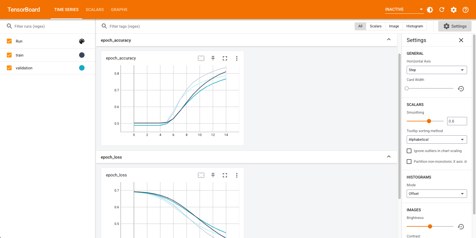
TensorBoard 를 사용하여 손실 및 정확도를 포함한 메트릭을 시각화합니다. tf.keras.callbacks.TensorBoard 를 만듭니다.
tensorboard_callback = tf.keras.callbacks.TensorBoard(log_dir="logs")
Adam 옵티마이저와 BinaryCrossentropy 손실을 사용하여 모델을 컴파일하고 훈련합니다.
model.compile(optimizer='adam',
              loss=tf.keras.losses.BinaryCrossentropy(from_logits=True),
              metrics=['accuracy'])
model.fit(
    train_ds,
    validation_data=val_ds,
    epochs=15,
    callbacks=[tensorboard_callback])
Epoch 1/15
20/20 [==============================] - 2s 71ms/step - loss: 0.6910 - accuracy: 0.5028 - val_loss: 0.6878 - val_accuracy: 0.4886
Epoch 2/15
20/20 [==============================] - 1s 57ms/step - loss: 0.6838 - accuracy: 0.5028 - val_loss: 0.6791 - val_accuracy: 0.4886
Epoch 3/15
20/20 [==============================] - 1s 58ms/step - loss: 0.6726 - accuracy: 0.5028 - val_loss: 0.6661 - val_accuracy: 0.4886
Epoch 4/15
20/20 [==============================] - 1s 58ms/step - loss: 0.6563 - accuracy: 0.5028 - val_loss: 0.6481 - val_accuracy: 0.4886
Epoch 5/15
20/20 [==============================] - 1s 58ms/step - loss: 0.6343 - accuracy: 0.5061 - val_loss: 0.6251 - val_accuracy: 0.5066
Epoch 6/15
20/20 [==============================] - 1s 58ms/step - loss: 0.6068 - accuracy: 0.5634 - val_loss: 0.5982 - val_accuracy: 0.5762
Epoch 7/15
20/20 [==============================] - 1s 58ms/step - loss: 0.5752 - accuracy: 0.6405 - val_loss: 0.5690 - val_accuracy: 0.6386
Epoch 8/15
20/20 [==============================] - 1s 58ms/step - loss: 0.5412 - accuracy: 0.7036 - val_loss: 0.5390 - val_accuracy: 0.6850
Epoch 9/15
20/20 [==============================] - 1s 59ms/step - loss: 0.5064 - accuracy: 0.7479 - val_loss: 0.5106 - val_accuracy: 0.7222
Epoch 10/15
20/20 [==============================] - 1s 59ms/step - loss: 0.4734 - accuracy: 0.7774 - val_loss: 0.4855 - val_accuracy: 0.7430
Epoch 11/15
20/20 [==============================] - 1s 59ms/step - loss: 0.4432 - accuracy: 0.7971 - val_loss: 0.4636 - val_accuracy: 0.7570
Epoch 12/15
20/20 [==============================] - 1s 58ms/step - loss: 0.4161 - accuracy: 0.8155 - val_loss: 0.4453 - val_accuracy: 0.7674
Epoch 13/15
20/20 [==============================] - 1s 59ms/step - loss: 0.3921 - accuracy: 0.8304 - val_loss: 0.4303 - val_accuracy: 0.7780
Epoch 14/15
20/20 [==============================] - 1s 61ms/step - loss: 0.3711 - accuracy: 0.8398 - val_loss: 0.4181 - val_accuracy: 0.7884
Epoch 15/15
20/20 [==============================] - 1s 58ms/step - loss: 0.3524 - accuracy: 0.8493 - val_loss: 0.4082 - val_accuracy: 0.7948
<keras.callbacks.History at 0x7fca579745d0>
이 접근 방식을 사용하면 모델은 약 78%의 유효성 검사 정확도에 도달합니다(훈련 정확도가 더 높기 때문에 모델이 과적합됨).
모델 요약을 살펴보고 모델의 각 계층에 대해 자세히 알아볼 수 있습니다.
model.summary()
Model: "sequential"
_________________________________________________________________
 Layer (type)                Output Shape              Param #
=================================================================
 text_vectorization (TextVec  (None, 100)              0
 torization)

 embedding (Embedding)       (None, 100, 16)           160000

 global_average_pooling1d (G  (None, 16)               0
 lobalAveragePooling1D)

 dense (Dense)               (None, 16)                272

 dense_1 (Dense)             (None, 1)                 17

=================================================================
Total params: 160,289
Trainable params: 160,289
Non-trainable params: 0
_________________________________________________________________
TensorBoard에서 모델 측정항목을 시각화합니다.
#docs_infra: no_execute
%load_ext tensorboard
%tensorboard --logdir logs
훈련된 단어 임베딩을 검색하고 디스크에 저장
다음으로 훈련 중에 학습한 단어 임베딩을 검색합니다. 임베딩은 모델의 임베딩 레이어의 가중치입니다. 가중치 행렬의 모양은 (vocab_size, embedding_dimension) 입니다.
get_layer() 및 get_weights() ) 를 사용하여 모델에서 가중치를 가져옵니다. get_vocabulary() 함수는 한 줄에 하나의 토큰으로 메타데이터 파일을 빌드하는 어휘를 제공합니다.
weights = model.get_layer('embedding').get_weights()[0]
vocab = vectorize_layer.get_vocabulary()
디스크에 가중치를 씁니다. 임베딩 프로젝터 를 사용하려면 두 개의 파일을 탭으로 구분된 형식으로 업로드해야 합니다. 벡터 파일(임베딩 포함)과 메타 데이터 파일(단어 포함)입니다.
out_v = io.open('vectors.tsv', 'w', encoding='utf-8')
out_m = io.open('metadata.tsv', 'w', encoding='utf-8')

for index, word in enumerate(vocab):
  if index == 0:
    continue  # skip 0, it's padding.
  vec = weights[index]
  out_v.write('\t'.join([str(x) for x in vec]) + "\n")
  out_m.write(word + "\n")
out_v.close()
out_m.close()
Colaboratory 에서 이 튜토리얼을 실행하는 경우 다음 스니펫을 사용하여 이러한 파일을 로컬 시스템에 다운로드할 수 있습니다(또는 파일 브라우저, 보기 -> 목차 -> 파일 브라우저 사용).
try:
  from google.colab import files
  files.download('vectors.tsv')
  files.download('metadata.tsv')
except Exception:
  pass
임베딩 시각화
임베딩을 시각화하려면 임베딩 프로젝터에 업로드하십시오.
임베딩 프로젝터 를 엽니다(로컬 TensorBoard 인스턴스에서도 실행할 수 있음).
"데이터 로드"를 클릭합니다.
위에서 생성한 두 개의 파일(
vecs.tsv및meta.tsv)을 업로드합니다.
학습한 임베딩이 이제 표시됩니다. 단어를 검색하여 가장 가까운 이웃을 찾을 수 있습니다. 예를 들어 "아름다운"을 검색해 보십시오. '멋지다'는 이웃을 볼 수 있습니다.
다음 단계
이 튜토리얼에서는 작은 데이터 세트에서 단어 임베딩을 처음부터 훈련하고 시각화하는 방법을 보여주었습니다.
Word2Vec 알고리즘을 사용하여 단어 임베딩을 훈련하려면 Word2Vec 자습서를 시도하십시오.
고급 텍스트 처리에 대해 자세히 알아보려면 언어 이해를 위한 변환기 모델을 읽어보세요.