Voir sur TensorFlow.org

Exécuter dans Google Colab

Voir sur GitHub

Télécharger le cahier

Voir le modèle TF Hub

TF-Hub est une plateforme pour partager l' expertise d'apprentissage de la machine emballée dans des ressources réutilisables, des modules notamment pré-formés. Dans ce didacticiel, nous utiliserons un module d'intégration de texte TF-Hub pour former un classificateur de sentiments simple avec une précision de base raisonnable. Nous soumettrons ensuite les prédictions à Kaggle.

Pour plus de détails tutoriel sur la classification de texte avec TF-Hub et d' autres mesures pour améliorer la précision, jetez un oeil à la classification du texte avec TF-Hub .

Installer

pip install -q kaggle

import tensorflow as tf
import tensorflow_hub as hub
import matplotlib.pyplot as plt
import numpy as np
import pandas as pd
import seaborn as sns
import zipfile

from sklearn import model_selection

Depuis ce tutoriel va utiliser un ensemble de données de Kaggle, il faut créer une API jeton pour votre compte Kaggle et de le télécharger à l'environnement Colab.

import os
import pathlib

# Upload the API token.
def get_kaggle():
  try:
    import kaggle
    return kaggle
  except OSError:
    pass

  token_file = pathlib.Path("~/.kaggle/kaggle.json").expanduser()
  token_file.parent.mkdir(exist_ok=True, parents=True)

  try:
    from google.colab import files
  except ImportError:
    raise ValueError("Could not find kaggle token.")

  uploaded = files.upload()
  token_content = uploaded.get('kaggle.json', None)
  if token_content:
    token_file.write_bytes(token_content)
    token_file.chmod(0o600)
  else:
    raise ValueError('Need a file named "kaggle.json"')

  import kaggle
  return kaggle


kaggle = get_kaggle()

Commencer

Données

Nous allons essayer de résoudre le Sentiment Analysis Film Critiques sur la tâche de Kaggle. L'ensemble de données se compose de sous-phrases syntaxiques des critiques de films Rotten Tomatoes. La tâche est d'étiqueter les expressions comme positif ou négatif sur l'échelle de 1 à 5.

Vous devez accepter les règles de la concurrence avant de pouvoir utiliser l'API pour télécharger les données.

SENTIMENT_LABELS = [
    "negative", "somewhat negative", "neutral", "somewhat positive", "positive"
]

# Add a column with readable values representing the sentiment.
def add_readable_labels_column(df, sentiment_value_column):
  df["SentimentLabel"] = df[sentiment_value_column].replace(
      range(5), SENTIMENT_LABELS)

# Download data from Kaggle and create a DataFrame.
def load_data_from_zip(path):
  with zipfile.ZipFile(path, "r") as zip_ref:
    name = zip_ref.namelist()[0]
    with zip_ref.open(name) as zf:
      return pd.read_csv(zf, sep="\t", index_col=0)


# The data does not come with a validation set so we'll create one from the
# training set.
def get_data(competition, train_file, test_file, validation_set_ratio=0.1):
  data_path = pathlib.Path("data")
  kaggle.api.competition_download_files(competition, data_path)
  competition_path = (data_path/competition)
  competition_path.mkdir(exist_ok=True, parents=True)
  competition_zip_path = competition_path.with_suffix(".zip")

  with zipfile.ZipFile(competition_zip_path, "r") as zip_ref:
    zip_ref.extractall(competition_path)

  train_df = load_data_from_zip(competition_path/train_file)
  test_df = load_data_from_zip(competition_path/test_file)

  # Add a human readable label.
  add_readable_labels_column(train_df, "Sentiment")

  # We split by sentence ids, because we don't want to have phrases belonging
  # to the same sentence in both training and validation set.
  train_indices, validation_indices = model_selection.train_test_split(
      np.unique(train_df["SentenceId"]),
      test_size=validation_set_ratio,
      random_state=0)

  validation_df = train_df[train_df["SentenceId"].isin(validation_indices)]
  train_df = train_df[train_df["SentenceId"].isin(train_indices)]
  print("Split the training data into %d training and %d validation examples." %
        (len(train_df), len(validation_df)))

  return train_df, validation_df, test_df


train_df, validation_df, test_df = get_data(
    "sentiment-analysis-on-movie-reviews",
    "train.tsv.zip", "test.tsv.zip")

Split the training data into 140315 training and 15745 validation examples.

train_df.head(20)

Former un modèle

class MyModel(tf.keras.Model):
  def __init__(self, hub_url):
    super().__init__()
    self.hub_url = hub_url
    self.embed = hub.load(self.hub_url).signatures['default']
    self.sequential = tf.keras.Sequential([
      tf.keras.layers.Dense(500),
      tf.keras.layers.Dense(100),
      tf.keras.layers.Dense(5),
    ])

  def call(self, inputs):
    phrases = inputs['Phrase'][:,0]
    embedding = 5*self.embed(phrases)['default']
    return self.sequential(embedding)

  def get_config(self):
    return {"hub_url":self.hub_url}

model = MyModel("https://tfhub.dev/google/nnlm-en-dim128/1")
model.compile(
    loss = tf.losses.SparseCategoricalCrossentropy(from_logits=True),
    optimizer=tf.optimizers.Adam(), 
    metrics = [tf.keras.metrics.SparseCategoricalAccuracy(name="accuracy")])

history = model.fit(x=dict(train_df), y=train_df['Sentiment'],
          validation_data=(dict(validation_df), validation_df['Sentiment']),
          epochs = 25)

Epoch 1/25
4385/4385 [==============================] - 16s 3ms/step - loss: 1.0237 - accuracy: 0.5869 - val_loss: 1.0023 - val_accuracy: 0.5870
Epoch 2/25
4385/4385 [==============================] - 15s 3ms/step - loss: 0.9995 - accuracy: 0.5941 - val_loss: 0.9903 - val_accuracy: 0.5952
Epoch 3/25
4385/4385 [==============================] - 15s 3ms/step - loss: 0.9946 - accuracy: 0.5967 - val_loss: 0.9811 - val_accuracy: 0.6011
Epoch 4/25
4385/4385 [==============================] - 15s 3ms/step - loss: 0.9924 - accuracy: 0.5971 - val_loss: 0.9851 - val_accuracy: 0.5935
Epoch 5/25
4385/4385 [==============================] - 15s 3ms/step - loss: 0.9912 - accuracy: 0.5988 - val_loss: 0.9896 - val_accuracy: 0.5934
Epoch 6/25
4385/4385 [==============================] - 15s 3ms/step - loss: 0.9896 - accuracy: 0.5984 - val_loss: 0.9810 - val_accuracy: 0.5936
Epoch 7/25
4385/4385 [==============================] - 15s 3ms/step - loss: 0.9892 - accuracy: 0.5978 - val_loss: 0.9845 - val_accuracy: 0.5994
Epoch 8/25
4385/4385 [==============================] - 15s 3ms/step - loss: 0.9889 - accuracy: 0.5996 - val_loss: 0.9772 - val_accuracy: 0.6015
Epoch 9/25
4385/4385 [==============================] - 15s 3ms/step - loss: 0.9880 - accuracy: 0.5992 - val_loss: 0.9798 - val_accuracy: 0.5991
Epoch 10/25
4385/4385 [==============================] - 15s 3ms/step - loss: 0.9879 - accuracy: 0.6002 - val_loss: 0.9869 - val_accuracy: 0.5935
Epoch 11/25
4385/4385 [==============================] - 15s 3ms/step - loss: 0.9878 - accuracy: 0.5998 - val_loss: 0.9790 - val_accuracy: 0.5985
Epoch 12/25
4385/4385 [==============================] - 14s 3ms/step - loss: 0.9871 - accuracy: 0.5999 - val_loss: 0.9845 - val_accuracy: 0.5964
Epoch 13/25
4385/4385 [==============================] - 15s 3ms/step - loss: 0.9871 - accuracy: 0.6001 - val_loss: 0.9800 - val_accuracy: 0.5947
Epoch 14/25
4385/4385 [==============================] - 15s 3ms/step - loss: 0.9873 - accuracy: 0.6001 - val_loss: 0.9810 - val_accuracy: 0.5934
Epoch 15/25
4385/4385 [==============================] - 14s 3ms/step - loss: 0.9865 - accuracy: 0.5988 - val_loss: 0.9824 - val_accuracy: 0.5898
Epoch 16/25
4385/4385 [==============================] - 15s 3ms/step - loss: 0.9865 - accuracy: 0.5993 - val_loss: 0.9779 - val_accuracy: 0.5974
Epoch 17/25
4385/4385 [==============================] - 15s 3ms/step - loss: 0.9866 - accuracy: 0.5991 - val_loss: 0.9785 - val_accuracy: 0.5972
Epoch 18/25
4385/4385 [==============================] - 15s 3ms/step - loss: 0.9863 - accuracy: 0.6001 - val_loss: 0.9803 - val_accuracy: 0.5991
Epoch 19/25
4385/4385 [==============================] - 16s 4ms/step - loss: 0.9863 - accuracy: 0.5996 - val_loss: 0.9773 - val_accuracy: 0.5957
Epoch 20/25
4385/4385 [==============================] - 15s 3ms/step - loss: 0.9862 - accuracy: 0.5995 - val_loss: 0.9744 - val_accuracy: 0.6009
Epoch 21/25
4385/4385 [==============================] - 15s 3ms/step - loss: 0.9861 - accuracy: 0.5997 - val_loss: 0.9787 - val_accuracy: 0.5968
Epoch 22/25
4385/4385 [==============================] - 15s 3ms/step - loss: 0.9855 - accuracy: 0.5998 - val_loss: 0.9794 - val_accuracy: 0.5976
Epoch 23/25
4385/4385 [==============================] - 14s 3ms/step - loss: 0.9861 - accuracy: 0.5998 - val_loss: 0.9778 - val_accuracy: 0.5966
Epoch 24/25
4385/4385 [==============================] - 15s 3ms/step - loss: 0.9860 - accuracy: 0.5999 - val_loss: 0.9831 - val_accuracy: 0.5912
Epoch 25/25
4385/4385 [==============================] - 14s 3ms/step - loss: 0.9858 - accuracy: 0.5999 - val_loss: 0.9780 - val_accuracy: 0.5977

Prédiction

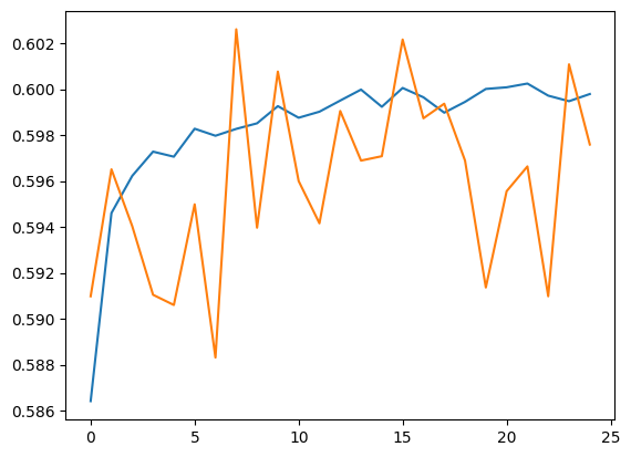
Exécutez des prédictions pour l'ensemble de validation et l'ensemble d'entraînement.

plt.plot(history.history['accuracy'])
plt.plot(history.history['val_accuracy'])

[<matplotlib.lines.Line2D at 0x7f62684da090>]

train_eval_result = model.evaluate(dict(train_df), train_df['Sentiment'])
validation_eval_result = model.evaluate(dict(validation_df), validation_df['Sentiment'])

print(f"Training set accuracy: {train_eval_result[1]}")
print(f"Validation set accuracy: {validation_eval_result[1]}")

4385/4385 [==============================] - 14s 3ms/step - loss: 0.9834 - accuracy: 0.6007
493/493 [==============================] - 1s 2ms/step - loss: 0.9780 - accuracy: 0.5977
Training set accuracy: 0.6006770730018616
Validation set accuracy: 0.5976500511169434

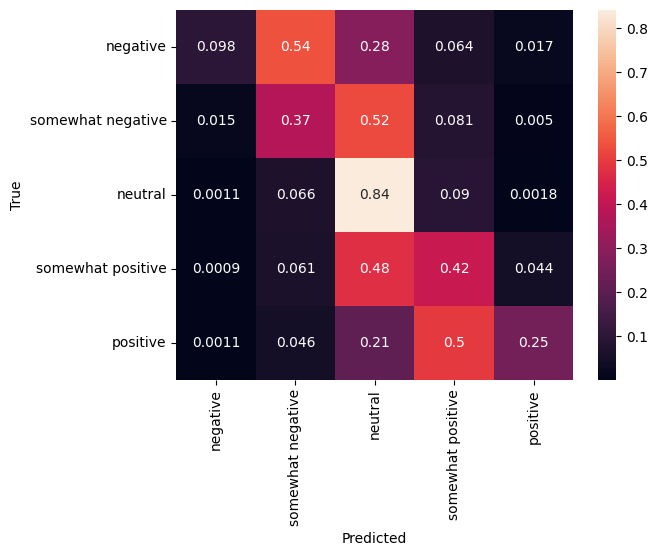
Matrice de confusion

Une autre statistique très intéressante, surtout pour les problèmes multiclassent, est la matrice de confusion . La matrice de confusion permet de visualiser la proportion d'exemples correctement et incorrectement étiquetés. Nous pouvons facilement voir à quel point notre classificateur est biaisé et si la distribution des étiquettes a du sens. Idéalement, la plus grande fraction de prédictions devrait être distribuée le long de la diagonale.

predictions = model.predict(dict(validation_df))
predictions = tf.argmax(predictions, axis=-1)
predictions

<tf.Tensor: shape=(15745,), dtype=int64, numpy=array([1, 1, 2, ..., 2, 2, 2])>

cm = tf.math.confusion_matrix(validation_df['Sentiment'], predictions)
cm = cm/cm.numpy().sum(axis=1)[:, tf.newaxis]

sns.heatmap(
    cm, annot=True,
    xticklabels=SENTIMENT_LABELS,
    yticklabels=SENTIMENT_LABELS)
plt.xlabel("Predicted")
plt.ylabel("True")

Text(32.99999999999999, 0.5, 'True')

Nous pouvons facilement soumettre les prédictions à Kaggle en collant le code suivant dans une cellule de code et en l'exécutant :

test_predictions = model.predict(dict(test_df))
test_predictions = np.argmax(test_predictions, axis=-1)

result_df = test_df.copy()

result_df["Predictions"] = test_predictions

result_df.to_csv(
    "predictions.csv",
    columns=["Predictions"],
    header=["Sentiment"])
kaggle.api.competition_submit("predictions.csv", "Submitted from Colab",
                              "sentiment-analysis-on-movie-reviews")

Après la présentation, vérifiez le leaderboard pour voir comment vous avez fait.